


Executive Summary
Regulations often restrict the range of market choices available to consumers, yet they are promulgated without a quantitative analysis of that cost—a fundamental flaw in regulatory impact analysis. This paper fills the gap by supplying a portable choice-value factor. The factor compares value at the unconstrained mix with regulation-constrained value. That comparison is a quantity-index comparison of two mixes—the same comparison the national accounts use to measure real GDP. It depends on displacement and on the difficulty of substitution at a reference mix. It can be applied to regulations that fully prohibit objects that consumers might choose or rules that shift market shares without full elimination.
Demand responses can identify the substitution parameter by separating in-market switching from scale. Compliance prices or household-production loads can identify the same objects. The choice-value factor is a conditional, within-market private-value measure. Externalities, resource costs, and fiscal effects remain distinct cost-benefit items. Prior analyses of health-insurance and vehicle regulations illustrate the method.
Beyond regulatory impact analysis, quantifying the value of consumer choice provides a foundation for understanding how markets work and how constraints alter human welfare by translating observed choices into a quantitative reflection of the economic world.
Introduction: Consumer Choice Is Invoked but Rarely Valued
1.1 The missing number
Consider a regulation that changes the mix of vehicles that manufacturers can profitably offer and consumers can afford to buy. The regulation need not prohibit a particular model. A fleet-average standard can instead alter relative prices: vehicles that make compliance more difficult become more expensive, vehicles that make compliance easier become less expensive, and manufacturers change their product offerings in response. Consumers then purchase a different mix of technologies, sizes, power, range, carrying capacity, and other attributes. Some consumers may also postpone buying a new vehicle or retain an older one.
A regulatory analysis can count many consequences of that policy. It can estimate engineering costs, fuel savings, emissions, safety effects, tax consequences, and changes in the number of new vehicles sold. But what dollar choice value should be assigned when consumers are induced to move away from the product mix they would have selected in the absence of regulation?
The question is not whether consumers should be free to impose costs on others. A complete benefit-cost analysis must separately account for emissions, congestion, safety, adverse selection, fiscal effects, information failures, and any other external or institutional consequence. Nor does the existence of a private choice cost determine whether a policy is desirable. The narrower claim of this paper is that the private value of the choices displaced by policy is a real component of welfare and should be measured rather than silently assigned a value of zero.
Vehicle regulation offers an unusually useful place to begin. Under past federal greenhouse-gas and fuel-economy programs, manufacturers could meet a tighter fleet constraint partly by purchasing compliance credits. The price of a credit was therefore a market signal about the private cost of an additional unit of compliance. A 2020 Council of Economic Advisers report used public records of nearly $700 million in credit transactions and interpreted the observed prices as incorporating both the cost of producing more efficient vehicles and consumers’ willingness to buy them.1 The compliance credit price does not, by itself, answer the entire question posed in this paper. It is nevertheless an important revealed-preference observation: market participants paid for flexibility rather than making the full product-mix adjustment required in the absence of that flexibility.
The central analytical task is to connect such observations to a general measure of choice value. This paper does so with a choice-value factor (CVF). The CVF compares the value generated when consumers can obtain the value-maximizing product mix with the value generated under a constrained mix. Its magnitude depends on two economic objects:
- Displacement: how far the policy moves the market from the value-maximizing mix; and
- Difficulty of substitution: how rapidly value falls as the mix moves away from that optimum.
A third object - the size of the affected market - converts the factor into dollars. Put simply, the calculation asks:
How far are consumers pushed, how difficult is it for them to substitute, and how much spending or economic activity is affected?
That is the paper’s answer to the question in its title.
1.2 Consumer choice across the Trump policy agenda
Consumer choice is not confined to one agency or one policy domain. It has been an explicit objective of a broad range of Trump-administration actions. Executive Order 14154, for example, states a policy of eliminating the “electric vehicle mandate” and promoting “true consumer choice,” and separately calls for safeguarding the freedom to choose among appliances.2 Other actions concern who chooses health coverage, which insurance plans may be offered, where families educate their children, and which saving or investment vehicles workers can access. Table 1 lists selected examples.
The examples are not institutionally identical. Vehicle and appliance standards change the mix of attributes that can be supplied and the relative prices at which they are supplied. Health-coverage, education, and retirement policies often change whether an intermediary assigns a uniform option or households may sort among heterogeneous options. In both settings the private welfare object is the same: the value of optimizing over a larger feasible set rather than a constrained mix. Heterogeneous people and heterogeneous products are why that value is not zero. Some coverage rules also leave a product legally available but raise the household time and administrative effort required to use it. That household-production margin is the object of the short-term-plan analysis in CEA (2019).3
Table 1. Selected Trump-administration policies in which consumer choice is central
| Policy area | Representative action or policy | Principal choice margin | Connection to the measurement framework |
|---|---|---|---|
| Vehicles | EPA rescission of federal motor-vehicle GHG standards; NHTSA’s SAFE Vehicles Rule III proposal | Vehicle technology, fuel economy, performance, size, price, and timing of purchase | A public implementation example. A fleet constraint changes relative prices and the product mix. Credit prices, vehicle shares, and demand responses can reveal the difficulty and value of substitution. 4,5,6 |
| Health coverage | 2019 individual-coverage HRA rules; 2027 Marketplace Payment Notice | Coverage-segment and plan-menu choice | These policies change available coverage segments or plan menus. Enrollment shares and paired elasticities can be used to value a generic movement from one coverage option to two. 7,8,9 |
| Household appliances | Executive Order 14154 and DOE’s proposed revision of the appliance-standards Process Rule | Purchase price, energy use, performance, durability, cycle time, and product features | Efficiency standards can remove or reprice configurations. Product shares, market elasticities, and compliance behavior can identify the value of the displaced attributes. 10,11 |
| Education | Executive Order 14191; Education Freedom Tax Credit | School, provider, tutoring, scholarship, and educational setting | Families and educational settings differ. The welfare object is the gain from better matching, measured through enrollment diversion, willingness to travel or pay, and the quality of outside alternatives. 12,13 |
| Retirement saving | Executive Orders 14330 and 14403; TrumpIRA.gov | Account access, investment menu, portability, fees, risk, and expected return | These actions change the available menu or reduce the cost of locating and selecting an account. Participation and portfolio reallocations can reveal value, subject to fiduciary, information, and agency considerations. 14,15 |
Insurance applications require an additional separation. Adverse selection can change equilibrium premiums and cross-subsidies at the same time that a rule changes consumer choice. Holding behavior and real resource use fixed, changes in premiums and cross-subsidies are largely transfers. Adverse selection affects aggregate surplus insofar as it changes the insurance allocation—whether people obtain coverage, which plan they choose, how generous that coverage is, whether insurers participate, or what contracts they offer—or changes real administrative or medical-resource costs or tax-financing distortions. These selection effects belong on neighboring lines of equation (1), not inside the choice-value factor.
A single calibration should not be copied from vehicles to schools. Which alternatives are being compared, whether the preferred mix is observed or must be inferred, and which external terms belong on the ledger all differ. But they answer one question: when policy changes the feasible set, what is the effect on private value? The rest of this paper develops a tractable answer, with reference to federal precedents.
1.3 Choice value is a component of welfare
Private choice value is a component of a complete benefit-cost calculation. People hold knowledge about their own circumstances—habits, schedules, local constraints, and valuations—that a central regulator cannot observe. That knowledge is productive, and choice is how it gets used. If consumers are heterogeneous, a restriction that moves them from selected products to second-best alternatives reduces private value. An expansion of the feasible set produces a corresponding private gain. Both have a dollar magnitude, and both should be measured.
A complete benefit-cost calculation therefore takes the form
Equation (1) requires that private choice value be identified explicitly and kept distinct from the engineering cost of compliance, the number of products removed, and the external benefit that motivates the regulation. Signs of the other terms, and any overlap with private choice value, depend on the application.
1.4 Federal revealed-preference precedents
Two federal vehicle analyses, one federal health-insurance analysis, and national accounting, provide especially important precedents.
The first is the Council of Economic Advisers’ 2020 report, Estimating the Value of Deregulating Automobile Manufacturing Using Market Prices for Emissions Credits. The report treated compliance-credit prices as revealed-preference evidence about the private cost of tighter standards. Its economic interpretation combined production costs with the opportunity cost of inducing a vehicle mix different from the mix consumers would otherwise select.16 The report also emphasized convexity: as standards push the market farther from the preferred mix, additional increments of compliance become increasingly costly when high- and low-emissions vehicles are imperfect substitutes.
The second is Appendix 2 of NHTSA’s 2025 preliminary regulatory impact analysis for the proposed SAFE Vehicles Rule III. That appendix uses a constant-returns quantity index, denoted here by , to represent the value consumers obtain from low- and high-MPG vehicles. It interprets the elasticity of substitution as a measure of how easily consumers can be induced to switch between the two categories and labels its inverse economic content the difficulty of substitution.17 Its quadratic formula is the same local approximation as Section 2.5; the index could be CES, but need not be.18
NHTSA’s appendix also imposes a revealed-preference restriction that the private benefits of consumer choice are not negative.19 This is not a claim that every unregulated outcome is socially optimal. It is the narrower proposition that, holding the relevant prices, resources, and external effects conceptually separate, allowing optimization over a larger feasible set cannot reduce the maximized private value generated by that set.
A third is the Council of Economic Advisers’ 2019 report, Deregulating Health Insurance Markets: Value to Market Participants. That report analyzed the 2018 short-term, limited-duration insurance rule as a household-production reform. The preceding 2016 rule had not banned those plans. It had required enrollees to reapply, and insurers to underwrite, as often as every three months. The 2018 rule allowed a contract to be renewed for up to 36 months. CEA modeled the change as a reduction in load and hassle costs: enrollee time together with repeated underwriting, commissions, and other administration. Those extra costs are a social loss rather than a transfer. Enrollment responses identified an equivalent price reduction, with supporting evidence from the administrative share of short-term premiums and from the demand for three-month “four-packs” that had been used to spread the same costs over a longer period.20
Fourth, the quantity index in NHTSA’s appendix is not an ad hoc regulatory construct. It is the same object the Bureau of Economic Analysis uses to measure real GDP: a chained Fisher quantity index, the geometric mean of Laspeyres and Paasche quantity indexes.21,22 BEA’s motor-vehicle output provides a concrete illustration by aggregating component products that include autos and trucks. BEA uses purchasers’ price levels to weight and aggregate quantities. Because purchasers’ prices include resource costs and any compliance wedge, both the resource-cost line and the choice-value line of equation (1) are embedded in the index.
The difference between a regulatory impact analysis (RIA) of choice value and national accounting is a difference of information, not of concept. National accountants measure prices and quantities at two points in time; an RIA must project both actual and baseline behavior. A reliable RIA does not ignore a change in choice value that the national accounts would, in hindsight, record as a meaningful change in real output.
These precedents establish that choice value can be approached empirically rather than treated as an unmeasurable preference for variety. The three regulatory analyses show that the object can be estimated in an RIA; the national accounts show that the federal government already computes the underlying quantity-index formula.
1.5 Contributions and roadmap
This paper makes five contributions.
First, it defines a choice-value factor: the ratio of value generated at the optimized product mix to value generated at a constrained mix. That ratio is a real-output quantity-index comparison of two mixes, the comparison BEA makes when it measures real GDP. The factor also has a dual cost interpretation as the proportional increase in minimum expenditure required to reproduce a given amount of value under the constraint.
Second, it shows that a second-order approximation to the CVF depends on two ingredients: how far the policy displaces the market from the value-maximizing mix, and the elasticity of substitution evaluated at a reference point (Section 2.5). A ban is a corner special case of that displacement, not the generic policy. When both endpoint price-quantity pairs are measured, the ordinary Fisher quantity index factors into a scale factor and a substitution factor: the Laspeyres factor measures scale, and the remaining Paasche-to-Laspeyres ratio measures substitution (Section 2.7). Revealed preference bounds the CVF between one and the Laspeyres-to-Paasche ratio.
Third, it connects the substitution parameter to observable behavior. Hicks-Marshall derived-demand logic separates within-market substitution from contraction of the total market. The diversion ratio is the destination of that split — another inside segment, an outside option, or delayed purchase — a function of the same share, scale, and substitution objects, not a separate primitive.
Fourth, it organizes three empirical routes within the same framework. Route 1 identifies the local elasticity of substitution from paired demand elasticities. Routes 2 and 3 recover related objects—compliance-credit prices and household-production loads—that coincide with the CVF inputs only under additional assumptions, notably pass-through and a mapping from remaining-user hassle into substitution. CEA (2019) is the worked Route 3 precedent.
Fifth, it translates the framework into a reporting protocol for regulatory impact analysis: define the counterfactual, identify the mix and reference point, report route-specific evidence and pass-through assumptions, calculate the private choice-value line, and keep the rest of the ledger in equation (1) separate.
Section 2 defines and derives the CVF, including the eight-observation endpoint calculation in Section 2.7. Section 3 develops Route 1. Section 4 develops Routes 2 and 3 and compares all three. Section 5 provides a protocol for regulatory impact analysis. Section 6 concludes. Appendix A derives the curvature-elasticity identity behind the second-order approximation. Appendix B derives the composite-segment identification result and the bound that applies when only part of the complement is observed.
Quantifying the Value of Choice
2.1 Setup and normalizations
Consider two inputs, product segments, or institutional arrangements, denoted by and . The notation is intentionally portable. In the vehicle application, and can be two vehicle classes. In other applications, the same symbols can stand for two appliance configurations, two coverage arrangements, or two methods of producing a service valued by households, including a method that is more intensive in household time or in underwriting and administration. A rule that requires more frequent renewal is then a change in the relative cost of those methods, not a prohibition of the product.
Let
be the quantity or value produced by the mix. The function may be read as a production function, a quality-adjusted quantity index, or an aggregate representation of the value created when heterogeneous consumers sort between two alternatives. In the national accounts, a quantity index is how real GDP is measured. BEA implements that measurement with a chained Fisher formula that uses observed prices as weights on observed quantities. The CVF is the same index evaluated at the optimized mix relative to the constrained mix, rather than at one period’s realized mix relative to another’s.23 The maintained assumptions for the local calculation are summarized in Table 2.
Table 2. Maintained assumptions and normalizations for the benchmark CVF
| Item | Assumption or normalization | Economic role |
|---|---|---|
| Technology or value index | is increasing, concave, and differentiable in both quantities and exhibits constant returns | Homogeneity permits a unit-cost interpretation; concavity makes the optimized mix value-maximizing; differentiability permits a second-order approximation |
| Prices or premiums |
| This is a local normalization of input-quantity units |
| Total expenditure |
| Fixes the scale of the comparison so that only the mix varies |
| Constrained allocation | , with and | A binding constrained share. The corner is a special case, not the generic policy |
| Output normalization |
| Units so that constrained output is one for the comparison being drawn |
| Interior optimum |
| Ensures that the first-order condition equates marginal products at the optimized mix |
| Substitution parameter | is the elasticity of substitution evaluated at the chosen reference point | Summarizes local curvature, as in Section 2.5 |
Because is homogeneous, its marginal rate of substitution depends on the input ratio. Define
With prices normalized to one and total expenditure fixed at one, the freely chosen mix solves
If the optimum is interior, its first-order condition is
or, equivalently,
The constrained allocation produces one unit of value by normalization. The optimized mix produces
with a strict inequality whenever differs from a unique, strictly preferred interior optimum.
The choice-value factor is therefore
The quantity is the proportional extra value produced by allowing the mix to be chosen rather than requiring , measured relative to the normalized constrained output. A CVF of 1.04, for example, would mean that the optimized mix produces 4 percent more value from the same normalized expenditure than the constrained mix. When , (8) is the corner comparison . The empirical sections will determine the relevant values rather than assume them.
2.2 Geometry: distance and curvature
Define the one-dimensional function
The constrained point is . The optimized point is , and . Figure 1 plots this comparison.
The hollow marker at is the corner special case, drawn in the same units.
The graph identifies the two economic determinants of choice value.
The first is distance. If is close to , the restriction causes little reallocation. If is far from , the restriction forces a large change in the mix.
The second is curvature. A broad, nearly flat peak means that the alternatives are close substitutes: a sizable change in the mix produces relatively little loss of value. A sharply curved peak means that the alternatives are poor substitutes: moving the same distance from the optimum produces a larger loss.
Thus the CVF is not a count of menu items. It is the value consequence of a particular displacement, given the ease or difficulty of substitution.
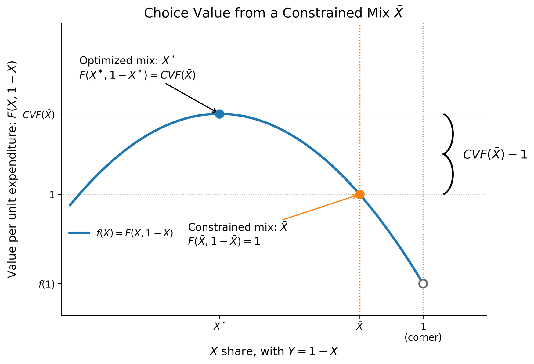
Figure 1. Choice value from a constrained mix .
Caption. With total expenditure and relative prices fixed, and with units chosen so that, the optimized mix generates units of value. The orange point is the binding constrained share. The hollow marker at is the special case of a ban. The magnitude of the factor depends on the displacement and on the curvature of between those mixes. A fleet-average standard, or any other partial constraint, is the orange comparison, not the corner.
2.3 The dual minimum-cost interpretation
The normalization also gives the CVF a useful cost interpretation.
Let be the minimum cost of producing units of value when the mix of and may be optimized. Let be the minimum cost when the mix is restricted to the constrained share . Because prices are one and expenditure is normalized to one, the unrestricted allocation produces units of value per dollar, whereas the restricted allocation produces one unit per dollar. Linear homogeneity then implies
It follows that
The same factor that measures the output gain from choice therefore measures the increase in cost caused by the constraint. The dollar cost can be written using either the unrestricted or constrained cost base:
Equation (12) is useful in applications because available data may correspond to either base. It also prevents a common scaling error. Multiplying by constrained expenditure is not the same as multiplying it by unrestricted minimum expenditure. The analyst should state which base is observed and use the corresponding expression.
2.4 The elasticity of substitution as local curvature
The remaining task is to express the curvature of in an economically interpretable way. Let denote the elasticity of substitution between and , evaluated at the optimized mix. Using the marginal rate of substitution in (3), define
The derivative is taken along an isoquant. A high means that the input ratio can change substantially with only a small change in relative marginal valuation; the alternatives are close substitutes. A low means that a substantial relative-price or marginal-valuation change is needed to induce the same change in the mix.
For the benchmark normalization, local curvature and the elasticity of substitution are related by
Appendix A derives (14) from the definition (13), linear homogeneity of , and the first-order condition (5). Concavity makes , while . Equation (14) is the bridge between the geometry and observable economic behavior.
2.5 The second-order choice-value approximation
Expand to second order around the optimum and evaluate it at the constrained share :
Because is the optimum, . Substituting (14) gives
The choice-value factor is the ratio of those heights. With the normalization and ,
Equation (17) is the paper’s basic quantitative expression. It requires the optimized share , the constrained share , and the elasticity of substitution at the reference point. It does not require the elasticity to be constant away from that point. The corner formula is the special case , which reduces the displacement term to .
A comparison of two constrained shares, and , is the ratio of two such factors, . That is the interior-to-interior object in Section 5; it is the same quadratic, not an adjacent construction.
Define
Then
For a sufficiently small displacement-curvature term,
Equations (14)–(20) use the elasticity of substitution at the reference point as a coefficient of local curvature. A CES function is one possible global function with constant elasticity, but no CES restriction is imposed here; the elasticity may vary with composition. NHTSA’s 2025 Appendix 2 makes the same distinction: its quadratic formula is a second-order approximation for a constant-returns quantity index, and the index could be CES but need not be.24
2.6 Economic interpretation and comparative statics
Table 3 summarizes the formula’s interpretation. Displacement is the policy margin. The elasticity of substitution is a characteristic of the alternatives; it is cross-application variation in , not a policy-induced change in the parameter, that changes the CVF for a given displacement.
A large market share is not a large value of choice, and a high own-segment elasticity is not : some of the response may be scale. Section 3 separates those responses. The value of choice need not be large merely because a product disappears, nor small merely because most consumers remain in the market. Diversion tells where they go; helps tell how far downhill they move.
2.7 Fisher Indexes and the Choice-Value Factor
Section 2.6 treats as a characteristic that differs across applications. A separate question, even within one application, is whether that elasticity is constant between the optimized mix and the constraint. Equation (17) evaluates it at the optimized mix. That is a reference-point choice, not an assertion that is constant over the entire interval between and .
Table 3. Comparative statics of the choice-value factor
| Source of variation | Economic interpretation | Effect on approximate , holding other terms fixed |
|---|---|---|
shrinks | The constrained mix is closer to the freely chosen mix | Decreases CVF toward 1 |
grows | The constraint requires a larger reallocation | Increases CVF |
| The comparison is rather than an interior share | A ban is a larger displacement than a partial constraint, holding fixed | Increases CVF relative to the interior comparison |
| Applications with higher | and are closer substitutes; value falls more slowly away from the optimum | Decreases CVF toward 1 |
| Applications with lower | Substitution is more difficult; a given displacement requires a larger compensating price change | Increases CVF |
| The relevant expenditure or cost base rises | More dollars are exposed to the same proportional distortion | Leaves CVF unchanged but increases the dollar value |
| The affected population rises | The same per-unit loss applies to more consumers, vehicles, or covered lives | Leaves CVF unchanged but increases aggregate value |
If substitution difficulty changes along the adjustment path, a local approximation constructed from information near one composition will differ from an approximation constructed near another composition. This is the familiar index-number issue represented by Laspeyres and Paasche measures: a finite change can be valued using weights or local relationships from the initial point, from the comparison point, or from a symmetric combination of the two. The economic event is the same; the local information used to approximate it differs.
The symmetric combination is Fisher’s ideal quantity index, the geometric mean of Laspeyres and Paasche. BEA uses chained Fisher indexes to measure real GDP and related aggregates.25,26 To make the orientation explicit, let superscript 0 denote the unconstrained allocation and 1 denote the constrained. At each endpoint, are the two purchaser prices and are the two quantities, for . The ordinary Laspeyres and Paasche quantity indexes are
These indexes rely on only eight numerical inputs: baseline prices and quantities and projections of prices and quantities under the policy. Moreover, the Fisher index is readily decomposed into scale and substitution factors:
In this decomposition, the Laspeyres factor measures the quantity change at baseline-price weights. The remaining radical measures the substitution effect. Multiplying both policy quantities by any common factor multiplies , , and by that factor but leaves their ratios unchanged. Thus, the substitution factor removes a proportional change in scale. The raw Fisher index contains both effects, whereas its substitution factor isolates the substitution effect.
For the CVF interpretation, both endpoint bundles must be generated by the same increasing, concave, linearly homogeneous ; the baseline mix must be value-maximizing after accounting for other distortions; and policy purchaser prices must support the policy bundle. Stable preferences and product definitions are also required. Under these maintained assumptions, homogeneity permits the equal-baseline-expenditure comparison to be written directly in the original quantities:
The CVF compares the value of those mixes at the same baseline-price expenditure. Revealed preference then gives
Under the same quadratic approximation to f used in (15)–(17), the CVF equals their arithmetic midpoint:
Equivalently, the proportional extra value of choice is half the proportional gap between Laspeyres and Paasche, measured relative to Paasche:
These equalities are exact if is quadratic over the comparison interval; when that quadratic is only a local approximation, the implied CVF is an approximation too.
No separate estimate of is needed to calculate the midpoint because the endpoint observations determine , which incorporates the effect of the regulation on the product mix and the revealed difficulty of substitution. The ratio is the upper bound, not the CVF itself.
In short, price and quantity projections and widely-used national accounting formulae are enough to calculate the Choice Value Factor. Indeed, the required price and quantity inputs may well be reported in RIAs that nonetheless left choice value unquantified.
2.8 From the formula to an empirical estimate
The CVF calculation requires a small set of inputs.
The remainder of the paper is organized around identification of these inputs. Route 1 (Section 3) uses paired demand elasticities to separate inside substitution from scale. Route 2 (Section 4.1) uses compliance-credit prices as the slope of constraint cost. Route 3 (Section 4.2) uses remaining-user time, hassle, and underwriting; CEA (2019) is the worked precedent. They are windows on the same two determinants in Figure 1. Equation (12) converts the factor into dollars.
Table 4. Ingredients for estimating the CVF
| Object | Interpretation | Candidate evidence |
|---|---|---|
| Share of the normalized mix allocated to at the value-maximizing reference allocation | Unconstrained or less-constrained market shares; policy simulations; pre-policy shares; experimental or quasi-experimental choices |
| Displacement between the optimized mix and the constrained share | Same sources as , with explicit definition of the counterfactual; only if the rule is a ban |
| Elasticity of substitution at reference composition | Compliance-market responses; paired own-price elasticities for an exhaustive two-part partition, or an own-segment elasticity together with a market elasticity; cross-price responses; diversion; household-production evidence on time, hassle, and administrative or underwriting effort |
| Prices & quantities | Laspeyres and Paasche quantity indexes form scale and substitution terms | RIA baseline and policy projections, market data, or a model that reports both price-quantity pairs |
or | Unrestricted or constrained minimum cost or expenditure base to which the factor applies | Vehicle expenditure, premium or compensation base, appliance expenditure, time and administrative loads, or another quality-adjusted resource base |
Route 1: Demand-Response Identification through Marshall’s Laws and Diversion
Section 2 expressed the choice-value factor in terms of displacement and a local elasticity of substitution. Those objects are not named in the data. This section develops Route 1, demand-response identification, through the Hicks-Marshall decomposition of an observed demand response. Routes 2 and 3 are developed in Section 4; neither is derived from Marshall’s laws.
Route 1 can be understood as a restatement of the Fisher index multiplicative decomposition from Section 2.7 in terms of derived demand. There, is the scale factor and is the substitution factor. The Hicks-Marshall identities separate an observed demand response into the sum of two elasticity terms: a scale term governed by the elasticity of total inside-market demand and a substitution term governed by the elasticity of substitution between the segments. Selecting one expression or another is largely a question of what price and quantity data are available.
3.1 Derived demand and the two responses to a segment price
Consider a market with three kinds of option:
- an inside segment ;
- the exhaustive collection of all other inside segments, denoted by , which may itself be a composite; and
- an outside option .
These are the same two arguments of the Section 2 aggregator , plus an outside option that Section 2 shut down by holding total inside expenditure fixed at one. In a vehicle application, and may be two classes of new vehicles and postponement, an older vehicle, or exit. In an insurance application, and may be two coverage arrangements and remaining uninsured or obtaining protection outside the measured market. The outside option is a destination of displaced demand.
A rise in the price of reduces its quantity. That reduction is not a single economic event. It is the sum of two responses.
The first is substitution, or switching. Some demand that leaves arrives at . Consumers stay in the inside market and change the mix. This is movement along an isoquant of , governed by the elasticity of substitution between and , written as .
The second is scale. Some demand that leaves does not arrive at . Total use of the inside market contracts as consumers delay, exit, or substitute into . This is movement off the unit-expenditure simplex that Section 2 used to isolate mix from scale. The size of that contraction is governed by the elasticity of total inside-market demand with respect to the inside price, written below. Figure 2 is the corresponding diagram.
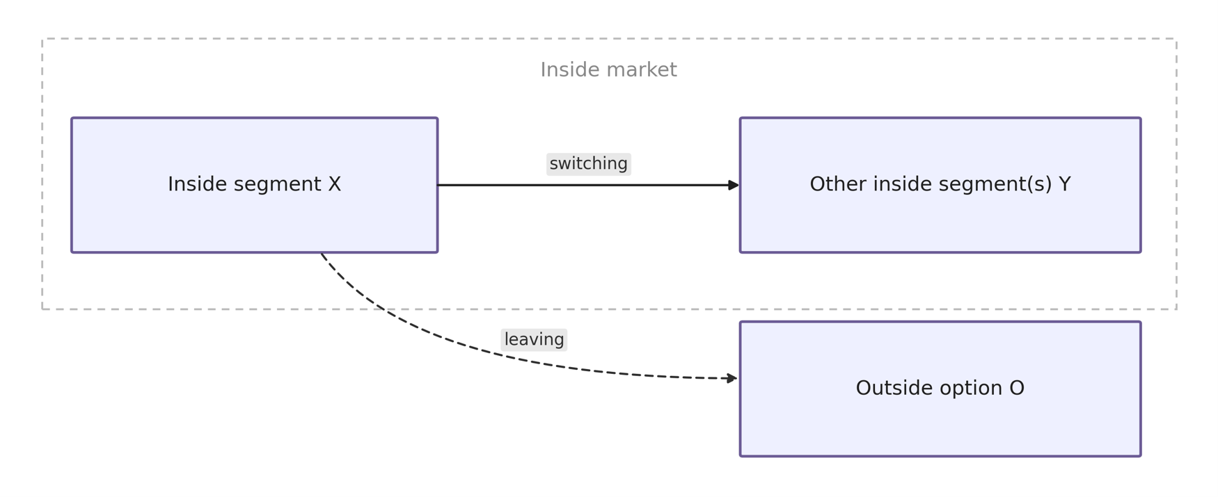
Figure 2. Substitution and scale responses to an increase in the price of .
Caption. The rectangle delimits the inside market; lies outside it, encompassing delay, a used durable, coverage or provision obtained outside the measured market, and informal provision. Segment ’s observed own-price elasticity is , and its share of inside expenditure is . A price increase for sends some demand to —substitution, the solid arrow, and movement along an isoquant of governed by —and some to —scale, the dashed arrow, and contraction governed by . The observed own-segment response is the sum of two effects: substitution contributes to , and scale contributes . The diversion ratios are the destination reading of the same Marshall objects, and , not the shares of those two additive terms. The elasticity of substitution is identified from that destination split, not from the own-segment response alone.
Section 2’s unit-expenditure normalization was the right device for defining the CVF, but it is the wrong device for reading an observed price response because the data do not hold scale fixed. The task here is to recover the substitution object of Section 2 from data in which substitution and scale are mixed.
3.2 Hicks-Marshall decomposition
Marshall’s laws of derived demand state that demand for an input or segment is more elastic when output demand is more elastic and when substitution toward cooperating inputs or segments is easier.27 Hicks gave the laws a quantitative form for a constant-returns, two-stage structure.28 The same structure is the natural companion of Section 2: a linearly homogeneous inside aggregator and a demand for the aggregator.
Let denote inside-market scale, and let be the corresponding unit-cost or price index. When is a composite of several other inside segments, hold their internal relative-price vector fixed and write . Define the composite quantity by , where is the quantity of primitive segment ; in the two-block notation below, denotes this composite price . Whether is primitive or composite, inside expenditure is . Write
Let be the elasticity of substitution between and , evaluated at the sample composition. Let
be the elasticity of total inside-market demand with respect to the inside price index. Demand slopes down, so . Let
be the own-price elasticities of the two inside blocks, each holding the other block’s price constant. Both elasticities are negative.
A price increase for then has the two effects already named. Holding inside scale constant, cost minimization on the aggregator reallocates toward . Under linear homogeneity, the Hicksian own-price elasticity of is . Holding relative inside prices constant, the rise in reduces . Shephard’s lemma implies that ’s contribution to the price index is its expenditure share, so this scale effect is . Adding the two effects, and writing the symmetric decomposition for , yields the benchmark identities
Equation (24) has the same form with any number of inside segments. For a focal segment , let denote its Allen-Uzawa elasticity of substitution with segment , and define
This is the expenditure-share-weighted average of ’s substitution elasticities with all other inside segments.29 For the exhaustive partition that takes as the quantity of and as the composite of , the in (24) is exactly . Both equations in (24), and therefore the identification formulas (25)–(28), remain exact when is the own-price elasticity of the complete composite with respect to . It is not the elasticity of one member of , nor a share-weighted average of the members’ individual own-price elasticities. Pairwise substitution elasticities may differ; no CES restriction is required. If relative prices within vary independently rather than proportionally, exact use of a single requires a linearly homogeneous, weakly separable subaggregate and its corresponding unit-cost index.
For this exhaustive two-block partition, the two equations contain two unknowns, and , once the share and the two own-price elasticities are observed. Two own-price elasticities therefore suffice. Adding the identities gives
and, when ,
The same pair also recovers the market elasticity,
Equation (26) is the operational mapping from the paired own-price elasticities of the exhaustive -versus- partition to the local curvature parameter of Section 2. The implied in (27) is a byproduct: it can be compared with an independent estimate of market demand when one is available. If , the benchmark implies , and the two own-price elasticities identify only the difference . Diversion, or a market-wide elasticity, is then needed to split that difference.
An alternative is one own-price elasticity and the market-wide elasticity. If is observed independently, (24) can be solved for from either segment:
This alternative is useful when only one segment elasticity is well measured, or when a market-demand estimate is more reliable than the second segment elasticity. If all three elasticities are observed, the system is overidentified: (25) is then a specification test rather than an identifying restriction.
Neither mapping is model-free. Table 5 states the maintained assumptions.
Several implications follow immediately.
First, a single own-segment elasticity cannot identify by itself. A more elastic own-segment response (more negative ) is consistent with easy inside substitution (large ) and with a more elastic scale response (more negative ). Those two cases have opposite consequences for the CVF. Easy inside substitution means that a given displacement of the mix is not very costly. A large scale response means that many displaced buyers are leaving the inside market rather than switching to a close inside substitute. Using one own-segment elasticity in place of in (17) therefore mixes the object the formula needs with an object it does not. The second elasticity—whether the exhaustive-composite elasticity or the market elasticity —is what separates the two.
Second, the implied is a local elasticity at the composition in the elasticity sample. That composition need not be the Section 2 reference point . As Section 2.7 emphasized, the analyst should report the composition at which is measured. Equations (26) and (28) do not convert a local elasticity into a globally constant one.
Third, the identity can be checked for internal consistency. Concavity and interior substitution require . In the two-own-price case, that is a restriction on , , and . In the alternative that uses , the data must satisfy (and ). Because the demand elasticities are negative, this is the requirement that each own-segment response be more elastic than its scale term. A violation is a warning that the inside market is mis-defined, that the elasticities mix horizons or price concepts, or that the two-stage structure is a poor description of the application.
Table 5. Maintained assumptions for the benchmark substitution-scale identity
| Item | Assumption | Role in (24)–(28) |
|---|---|---|
| Inside aggregator | Two-stage demand through a linearly homogeneous , with the exhaustive complement of | Permits a price index whose share weights are expenditure shares; a multi-segment is exact for proportional internal price changes, or under arbitrary internal price changes when it is a linearly homogeneous, weakly separable subaggregate |
| Substitution parameter | 𝜎>0 evaluated at the sample composition; for a multi-segment 𝑌, 𝜎=𝑋 | Local curvature between 𝑋 and its exhaustive complement (Section 2.5) |
| Identification | The own-price elasticities and of the exhaustive two-block partition, or one own-price elasticity and the market elasticity | The two identities in (24) contain two unknowns. Two block-level own-price elasticities identify when ; one own-price elasticity and identify at any interior share |
| Market elasticity | is the elasticity of the same inside aggregate whose shares enter ; it is not converted to an absolute value | Aligns the scale term with the market in which substitution is defined; the scale contribution in (24) is |
| Sign convention | , , and are signed elasticities (negative for ordinary demand); | Lets enter (24) as rather than as an absolute value with a minus sign in front |
| Price experiment | The other block’s price is held constant; a change in the price of composite scales all of its component prices proportionally | Isolates the derivatives that (24) decomposes and prevents an individual component elasticity from being mistaken for |
| Time horizon | , , and refer to the same horizon | Mixing short-run segment responses with long-run market responses biases |
| Competitive cost minimization | Inside quantities are consistent with cost minimization on given prices | Makes Shephard’s lemma and the Hicksian substitution term available |
The objects , , and in (22)–(28) are signed elasticities, not absolute values. Estimates already reported with a negative sign can be entered as reported. If a source reports an absolute value, enter it with a negative sign.
If only a subaggregate is observed, the second own-price elasticity generally yields a bound rather than point identification. Under a homogeneous nested benchmark in which substitution within is at least as easy as substitution between and , treating as though it were the entire complement produces an upper bound on the outer when , a lower bound when , and no bound on from those two elasticities when the shares are equal. Because the CVF in (17) decreases with over the admissible range, the corresponding CVF bound runs in the opposite direction. Appendix B derives the exact composite result and this partial- bound.
3.3 Diversion ratios and Route 1 implementation
Equation (24) determines not only the size of the own-segment response but also its destination. The industrial-organization diversion ratio is that destination split. It is a function of the Marshall objects , , and , not a separate primitive.30
Under the two-stage benchmark, the Marshallian cross-price elasticity of the complementary composite with respect to is . In expenditure units — or in quantity units after the Section 2 normalization that sets — the share of the value leaving that arrives at is therefore
Diversion to the outside option is the complementary ratio,
and the two destinations exhaust the loss from ,
The compact forms on the right of (29)–(30) still involve , but that elasticity is the left-hand side of (24). Substituting yields the fully reduced expressions in , , and alone.
Equations (29)–(30) are expenditure diversion, the object that lines up with the expenditure shares in (24). They coincide with the quantity ratio when and are measured in the same units, as they are after the Section 2 price normalization. When observed prices differ, a one-unit move from to is not a one-dollar move. The corresponding value-unit object is
which equals (29) under the benchmark. Quantity diversion is then times (29). Mixing quantity diversion from one study with expenditure shares from another is a specification error, not a robustness check. Second-choice surveys, assortment experiments, and price-based derivatives can also produce different diversion measures; they answer related but not identical questions and should not be treated as interchangeable without a stated mapping.31
Because (29)–(30) are a reading of (24), an observed diversion ratio is another estimator of , not information about a different parameter. Solving (29) for the substitution elasticity gives
which is identical to (28) when the benchmark holds. The practical use of having both formulas is diagnostic. If paired elasticities and diversion ratios, taken from consistent markets and horizons, imply materially different values of , the two-stage structure or the market definition should be revisited before either number is entered in (17).
Shares, elasticities, and diversion therefore jointly discipline :
- locates the composition at which the local elasticity is evaluated and weights the scale terms in (24);
- the own-price elasticities of the exhaustive -versus- partition identify and through (26)–(27) when the benchmark applies;
- alternatively, one own-price elasticity and identify through (28);
- is the destination reading of the same objects, (29)–(30), and identifies through (33) when one of or is observed; it tests the benchmark when both sources are available.
These objects belong to Route 1. Each route supplies the displacement and inputs that (17) requires. Neither Route 2 nor Route 3 is derived from Marshall’s laws.
Routes 2 and 3: Compliance Markets and Household Production
This section develops compliance-market evidence (4.1) and household-production evidence (4.2), then compares all three routes (4.3). The methods are complementary sources of evidence about , , and the non-premium cost of using a product.
4.1 Route 2: Compliance markets
Route 2 reads the dual of Figure 1. The data are credit prices rather than demand elasticities, so the identifying question is different. The welfare object recovered is the same.
Route 1 asks how an observed demand response splits between substitution and scale. Route 2 asks of the credit market:
What do firms pay to avoid one more unit of forced product-mix adjustment, and how does that shadow price change with the constraint?
A market price for a little more flexibility is the local slope of the cost of the constraint, not the choice-value factor itself. Combined with how that slope changes as the constraint tightens, and with how far the mix has been moved, it identifies the same curvature parameter that (17) requires. Integrating that shadow-price schedule, or inserting the implied and into (17), recovers the vertical brace on Figure 1, converted to dollars by (12). A producer credit price maps onto the consumer mix in Figure 1 only under a stated pass-through assumption.
The constraint and transferable credits
A product-mix regulation can leave every model legally available and still change the mix, by requiring that a sales-weighted average of some attribute—fuel economy, emissions, energy use—meet a standard. Manufacturers then comply by changing product attributes, by shifting the mix of products sold, or, when the program permits it, by using a credit.
Write the standard in its native units as a scalar , oriented so that a larger value is a tighter mix constraint. In the vehicle application, miles-per-gallon-equivalent units have that orientation: a tighter greenhouse-gas or fuel-economy standard raises and, equivalently, raises the minimum share of the more-compliant class. NHTSA’s Appendix 2 records that arithmetic: a fleet fuel-economy constraint is a constraint on the mix of low- and high-MPG vehicles.32 The same logic applies to an appliance standard that averages across a product class, or to any other averaging-and-trading rule that makes one configuration cheaper to sell by making another more expensive.
When the constraint is transferable, a firm that over-complies generates a credit and a firm that under-complies must acquire one. Credits may also be banked or borrowed across years when the rules allow it. When trading is frictionless, the industry faces a single shadow price of the constraint. CEA (2020) and NHTSA’s Appendix 2 read observed credit prices as that shadow value.33,34 Route 2 is available when policy creates such an instrument, or when an earlier period of trading left a usable price history. Historical prices identify substitution difficulty from the period in which trading occurred; current firm-specific shadow values depend on whether the constraint remains tradable.
A competitive credit price as a shadow price
Let be the minimized unit cost of producing one unit of the Section 2 aggregator when the mix must satisfy the standard . At the unconstrained, cost-minimizing standard , the mix is the optimized mix of Section 2. By the envelope theorem, the shadow price of tightening the standard is the derivative of that unit cost,
Under cost minimization and competitive trading in a well-functioning credit market, the observed credit price equals that shadow price:
Equation (35) rests on cost minimization, on trades that are informative about that minimum, and on matching the credit’s unit to the unit of . Table 6 states those assumptions.
If the cost of credits is passed through to consumer prices, also governs the relative prices that induce the mix in Figure 1. Products that make the constraint harder to meet sell at a premium; products that make it easier sell at a discount. CEA (2020) and NHTSA Appendix 2 adopt one-for-one pass-through, as did the agencies’ own regulatory impact analyses of the same programs.35 Under that assumption, the sales-weighted average effect of a stricter standard on retail prices is exactly the credit price, whether there are two product types or many. The many-vehicle identity is an adding-up result: specific models can sell above or below the standard, while the market average equals the standard, so the common price effect of tightening is .36 That is the bridge from a producer credit market to the consumer mix that Section 2 values.
Pass-through is an identifying assumption. If markups vary with the standard, or if only part of reaches retail prices, the credit price remains a shadow value on the supply side and the consumer-price wedge is a stated fraction of . The analyst should state the incidence assumption and, where the data permit, report how moves with alternative pass-through rates.
When purchasers' prices and quantities are observed at both the constrained and unconstrained mixes, the endpoint calculation in Section 2.7 separates the Laspeyres scale factor from the substitution factor. That calculation is available with or without a credit market and is a finite-change counterpart to Route 1's local scale-substitution decomposition. In a compliance application, purchaser prices also contain the shadow-price wedge and therefore provide a direct reading of Route 2's dual.
The purchasers’ prices in that BEA calculation contain the two neighboring lines of the welfare ledger in (1). With one-for-one pass-through, each price is a resource-cost component plus a compliance wedge. For the CAFE application, keep in miles per gallon, so a larger is tighter and . Define reciprocal fuel-economy units and their shadow price by
The exact CAFE price wedges and binding fleet constraint are then
Here and are the resource-cost components, while and are fuel consumption per mile. (If is a composite, and are the corresponding composites, at the internal relative prices already held fixed in Section 3.) A composition-only adjustment holds the unit count and vehicle attributes fixed. Differentiating the binding constraint gives . Because , weighting that mix change at purchasers’ prices therefore splits as
BEA’s quantity index embeds the sum because it weights quantities at purchasers’ prices. It does not publish the two terms as separate welfare accounts. An RIA should separate them: the first term is the change in resources associated with the composition shift; integrating the second term along the path of the standard gives the Route 2 unit-cost area in (39). Equation (12) converts that unit-cost difference to dollars on the appropriate base. The same binding-standard identity implies that the compliance wedges cancel in current-dollar output, , but they remain in the relative-price weights that split nominal output into the Fisher price and quantity indexes. That is why the CVF can be embedded in BEA’s real-output calculation even though BEA reports no separate choice-value series.
From the credit-price level and its slope to local curvature
Figure 1 shows the value gain relative to constrained output. Figure 3 draws its dual: the unit-cost loss from tightening the constraint away from the optimized mix.
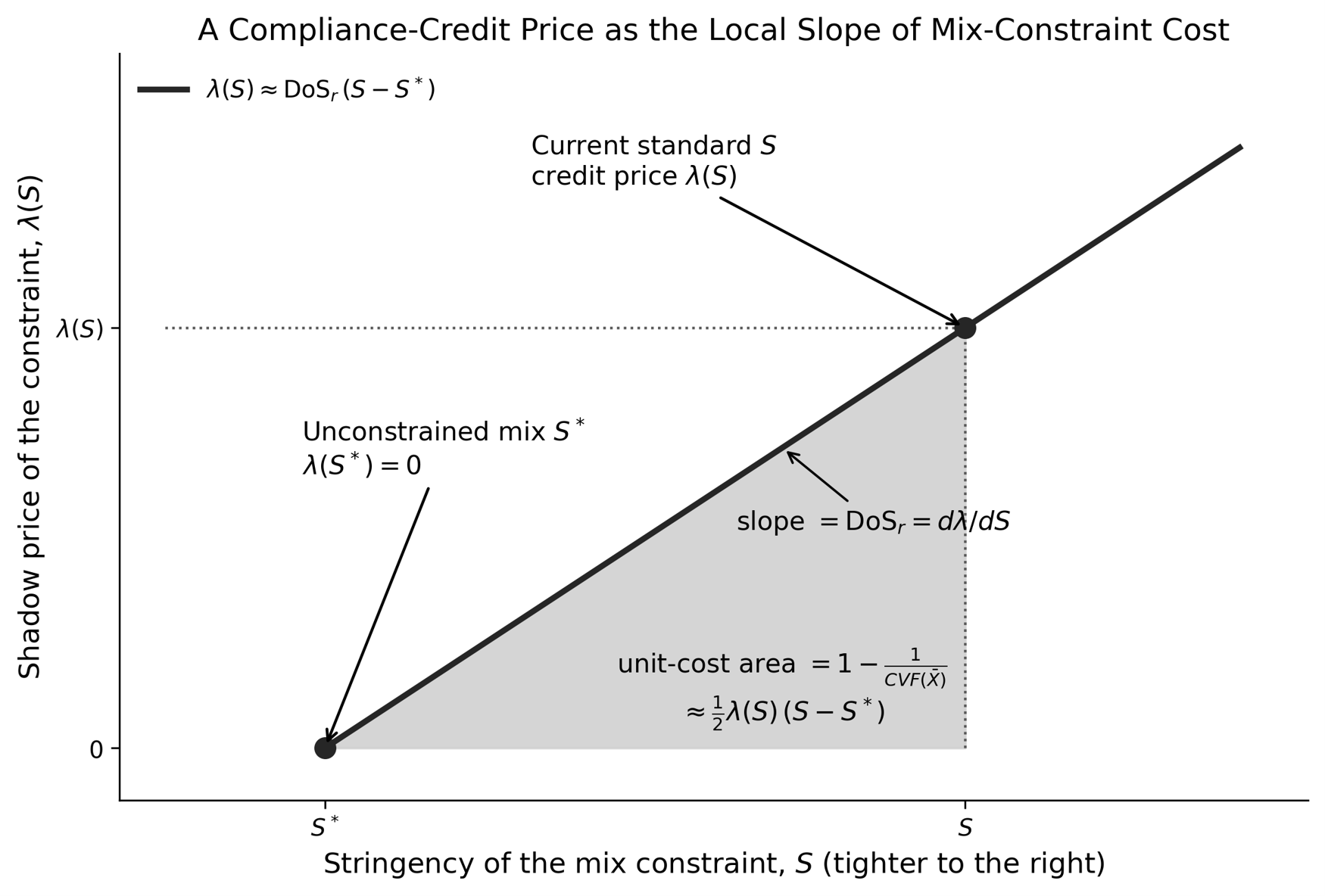
Figure 3. A compliance-credit price as the local slope of mix-constraint cost.
Caption. The horizontal axis measures constraint stringency, with the unconstrained mix at . The observed credit price is the height , and the slope is . Under the Section 2 constrained-unit-cost normalization, the shaded area is ; the triangle expression shown uses the locally linear- approximation.
To state the bridge between the figures precisely, the height in Figure 3 is not literally the slope of the blue value curve in Figure 1; it is the slope of the dual cost function. When a binding standard maps into the Section 2 mix as , the normalization gives , and therefore
The height in Figure 3 is thus the dual, unit-converted counterpart of the downward slope in Figure 1, while the slope in Figure 3 is the counterpart of Figure 1’s curvature. Because is unit cost, the shaded area is ; equation (12) converts that unit-cost difference into total dollars.
Because is minimized at , a local quadratic approximation to makes the shadow price linear in displacement. Define the difficulty of substitution at a stated reference point as the slope of that schedule:
If and are imperfect substitutes, is convex in the standard: additional increments of stringency are increasingly costly. That is the convexity emphasized in CEA (2020). NHTSA’s quadratic impact formula is likewise a local second-order approximation, with the elasticity evaluated at the unregulated composition.37
NHTSA’s Appendix 2 uses as the slope of the resource-and-opportunity-cost schedule and labels it the difficulty of substitution.38 A high means that a small further tightening of the standard raises the credit price a lot: manufacturers induce the required mix only with a large relative-price change, so the alternatives are poor substitutes. A low means that a tighter standard barely moves the credit price: substitution is easy. If the two classes are close substitutes, manufacturers meet a tighter standard by marketing the more-compliant class, and the schedule in Figure 3 is flat.
The elasticity of substitution in Section 2 is the inverse of that curvature, after a units conversion. Let be the factor that converts a change in the standard’s native units into the mix units in which is defined. Then
Equation (37) is the Route 2 counterpart of (26) and (28): it maps an observable schedule into the local curvature parameter of Section 2. The factor depends only on the reference composition and on the mapping from the standard to the mix. If the constraint is already a mix share, (14) and the dual cost function imply . If the constraint is a fleet average, also includes the derivative of that mix with respect to the standard—the arithmetic in NHTSA’s Equations A2-2 and A2-3. NHTSA writes the per-vehicle extra cost as ; the in that formula is this units factor evaluated at the unregulated composition.39
Two empirical readings of the same schedule follow.
A single credit price is a point on Figure 3. Given an estimate of or of the displacement , (36) yields the approximation .
The slope of the credit-price schedule, across two or more standards, identifies from two observed points:
CEA (2020) used this two-point reading. Anderson and Sallee estimated the marginal cost of tightening CAFE by one mile per gallon at about $18 per vehicle when the standard was 24.8 mpg, using the flex-fuel loophole.40 Tesla’s reported greenhouse-gas credit revenues, matched to EPA trade volumes, implied about $116 per mpg per vehicle (2018 dollars) at the 2012–2021 average standard of about 35 mpg.41 The implied slope is the that NHTSA then carried into its quadratic formula. This paper places that slope on the same curvature parameter that Route 1 recovers from paired elasticities.
The total extra unit cost of a standard relative to is the area under :
Under the linear schedule (36), the right-hand side of (39) is the shaded triangle in Figure 3. Equation (39) is the second-order remainder of the locally quadratic approximation to : linear corresponds to quadratic , not quadratic . Under the Section 2 constrained-unit-cost normalization, the exact unit-cost integral is . The identity applies to any binding , including an interior fleet constraint; equation (12) converts it to the equivalent dollar expression on either cost base.
A movement between two interior standards is the corresponding trapezoid, . That is the CEA and NHTSA calculation of the per-vehicle resource-and-opportunity-cost saving from relaxing a tighter rule toward a looser one. The conceptual distinction is the same one drawn for diversion in Section 3:
A credit price is the marginal cost of one more unit of the constraint. The total extra cost is the area under that schedule.
Mapping into the CVF
Once or and are in hand, (17) is the same formula as in Route 1. The reference-point discussion in Section 2.7 applies directly. Credit prices are observed at the mix that actually prevailed, which is a constrained mix if the standard binds. The implied is local to that composition. NHTSA accordingly denotes the elasticity at the unregulated fuel-economy composition by and allows it to vary as MPG changes.42 Report the composition at which and are measured. When prices exist at more than one standard, (38) can be computed on more than one interval, and the resulting range is ordinary index-number uncertainty.
NHTSA’s SAFE Vehicles Rule III proposal would eliminate inter-manufacturer CAFE credit trading beginning in model year 2028 if finalized as proposed.43 Historical credit prices still identify from the period in which trading occurred. Under a still-tight standard, eliminating trade raises the marginal cost of compliance for firms that had been net buyers, which is a steeper schedule in Figure 3. The historical slope remains evidence about substitution difficulty. The method is a revealed-preference reading of observed credit-market behavior.
Components of the observed shadow price
Equation (35) identifies a shadow price. The observed combines several economically distinct objects, each of which has its own place on the ledger:
- Engineering and production resource costs. Extra capital, materials, and assembly effort used to produce a more compliant product are real resource costs. They belong on the resource-cost line of (1).
- Opportunity cost of the mix. The value consumers forgo when induced to buy a different configuration is the choice-value object of Section 2. It is inside when meeting the standard requires a relative-price change.
- Scarcity rents and transfers. A payment from a credit buyer to a credit seller is a transfer. The price still reveals .
- Banking, borrowing, and expectations. Because credits can be saved and used later, the current price embeds expected future stringency, fuel prices, technology, and policy. CEA associated 2012–2016 Tesla prices with the 2012–2021 standards because credits earned in 2010–2016 could be used through 2021, and it treated those prices as conditional on expectations held at the time of the trades.44 A later change in expected policy moves the schedule in Figure 3.
- Credit-market power and thin trading. A large net buyer has an incentive to push the credit price down; a large net seller, to push it up. CEA noted that the average manufacturer is balanced between buying and selling over the full period, so the market price remains a reasonable estimate of sales-weighted average marginal cost, and would be a conservative estimate of that average if larger manufacturers were net buyers.45 Thin or non-arm’s-length trades, and prices imputed from one seller’s reported revenue, add measurement error around (35).
- Overlapping regulations. Vehicle manufacturers have faced both CAFE and greenhouse-gas constraints. CEA observed greenhouse-gas credit prices. If CAFE credits have independent value, the joint shadow value is the sum of the two prices.46
- Pass-through and markups. The incidence assumption determines how much of appears in consumer relative prices. Adding a constant seller markup would further add to the opportunity cost of a reduced quality-adjusted quantity, a point NHTSA flagged for comment.47
Convert the slope into with (37), combine it with in (17), and apply the resulting factor to the correct cost base in (12). Enter engineering costs on the resource-cost line of (1).
Table 6. Maintained assumptions for the credit-price identity
| Item | Assumption | Role in (34)–(39) |
|---|---|---|
| Constraint | A binding mix or fleet-average constraint with a defined physical unit | Supplies the argument of |
| Unit cost | is the minimized cost of one unit of subject to the standard | Makes an envelope shadow price |
| Cost minimization | Firms minimize private compliance cost | Equates the internal shadow value to the constraint |
| Competitive credit trading | Price-taking in the credit market, or a well-measured average of internal shadow values | Equates the observed credit price to in (35) |
| Pass-through | Stated incidence of into consumer relative prices | Connects a producer shadow value to the consumer mix that Section 2 values |
| Units factor | maps native units of into the mix units of | Converts into in (37) |
| Reference point | and are evaluated at a stated composition | Locates the composition at which the local slope is evaluated |
| Time horizon | The banking window, model years, and expectations embedded in the price are stated | Aligns with the constraint it is used to value |
Implementing Route 2
Gather:
- the constraint, its physical unit, and the mapping from that unit into the mix of and ;
- observed credit prices, transaction quantities, and the standards and model years to which those prices apply;
- whether the trades are arm’s-length, imputed from reported revenue, or internal transfers;
- the banking, borrowing, and averaging rules that determine the horizon over which a credit can be used;
- either an estimate of (or of the unconstrained mix) or a second point, so that (36) or (38) can be formed;
- the units factor when (17) is entered in elasticity units;
- the pass-through assumption, and any overlapping-program adjustment.
Classify and propagate uncertainty as in Section 3.3:
- identify whether each price is a recorded transaction, an imputation, an engineering analogue such as Anderson and Sallee’s loophole estimate, or an assumed value;
- distinguish prices formed under stable expected policy from prices formed around expected changes in the standard;
- exclude or bound thin, intra-firm, or settlement-valued trades;
- if CAFE and greenhouse-gas credit prices differ, add them for the joint shadow value, or treat a single-market price as a lower bound;
- if trading is later restricted, use historical as evidence about substitution difficulty and treat current firm-specific shadow values as at least as large for net buyers;
- convert into at a stated reference composition and enter that , with , in (17).
4.2 Route 3: Household production—time, hassle, and administrative effort
Route 3 reads a different observable, not a different welfare object. The data are non-premium inputs and the take-up response when those inputs change. The objects recovered are again displacement, local curvature, and a cost base.
Route 1 asks how an observed demand response splits between substitution and scale. Route 2 asks what firms pay to avoid one more unit of forced mix adjustment. Route 3 asks of remaining users of a product:
What non-premium inputs—household time, enrollee hassle, and firm underwriting or administration—are required to produce the service, and how does policy change those inputs for people who remain in the product?
Household production in this paper is those non-premium inputs used to produce the service. A duration or renewal rule that leaves the product legally available, but requires more frequent reapplication, is a change in the relative cost of two methods of producing it, not a prohibition. Extra enrollee time and extra underwriting, commissions, and administration are a social loss, not a transfer. Household production is not a synonym for market exit, remaining uninsured, or “household production of financial protection” by leaving the measured market. Those outside alternatives remain the Section 3 diversion destination ; they must still be valued, and they are not this estimand.
Remaining-user inputs as a full price
Let the two alternatives in Section 2 be two methods of producing the same service, or two quality versions of it. One method is more intensive in household time, enrollee hassle, or firm underwriting and administration. Write the load on that more burdensome version as , in dollars per unit, and write its full price as
The premium or sticker price is only part of the cost of using the version. Policy can change while leaving the product in the choice set: more frequent reapplication, a shorter maximum term that resets deductibles, additional documentation, or repeated underwriting. A lower is then a lower full price of that version. People who would have used the product either way still pay the extra load when is high. People at the margin switch in or out as the load changes.
An observed enrollment or take-up response, combined with an own-price elasticity of that version, identifies the equivalent change in full price. Let be that elasticity, and let be the proportional change in use of the version when the load changes. Then
Equation (41) is the Route 3 counterpart of (26) and (35): it maps an observable quantity response into a dollar object that (17) and (12) can use. If is defined with respect to the premium rather than the full price, replace with . A constant-semielasticity implementation of the same idea replaces with a level change scaled by a semi-elasticity, which is the form CEA (2019) used. Either implementation requires that and the enrollment change refer to the same version, the same horizon, and the same price concept. A transferred elasticity is a maintained assumption, not a robustness check.
The three objects in (41) overidentify one another, as the two own-price elasticities and do in Route 1. Observed take-up and an elasticity identify . A measured load—from administrative cost shares, time-use, or underwriting frequency—and an elasticity identify displacement. A measured load and observed take-up identify the elasticity, and therefore local curvature. Disagreement among those three readings is a specification warning, not a menu of alternative estimands.
The extra resource cost imposed on remaining users by a higher load is the rectangle
where is the quantity that would have been used at both the high-load and low-load full prices, and is an increase in load. Switchers’ surplus is the ordinary triangle associated with a relative-price change: approximately times the quantity displaced, if demand is locally linear. Newly insured people, or people who leave for the outside option, are a scale response. They belong in the diversion accounting of Section 3. They are not the remaining-user rectangle (42).
Lead example: short-term-plan duration
The 2016 short-term, limited-duration insurance rule did not technically ban the product. It limited the duration of a contract to less than three months, so that enrollees had to reapply, and insurers to underwrite, as often as every three months. Deductibles could reset, and coverage could lapse between contracts. The 2018 rule allowed an initial contract of less than twelve months and renewal of that contract for up to 36 months. CEA modeled both the duration restriction and the limited term as an addition to load and hassle costs—enrollee time together with repeated underwriting, sales commissions, and other administration—and compared high-loaded short-term coverage under the 2016 rule with low-loaded coverage under the 2018 rule.48
Those extra costs are a social loss rather than a transfer. The comparison with the individual-mandate penalty is the operational distinction. A penalty paid to the Treasury is a transfer plus whatever distortion it creates. Repeated reapplication and underwriting consume real resources. Reducing them is a social gain even for people who would have been in the product either way, and even if no one switched.
Enrollment responses identified the equivalent price change. CEA combined a projected increase in short-term enrollment with an own-premium elasticity of , transferred from a study of plan choice on the California and Washington ACA exchanges, in a constant-semielasticity demand function.49 The implied equivalent load reduction was $1,218 per enrollee. Two supporting observations discipline that magnitude. First, estimates that administration accounted for about half of short-term premiums imply considerable scope for spreading the fixed cost of underwriting, commissions, and other policy administration over a longer contract.50 Second, even before the 2018 rule, some insurers sold “four-packs” of three-month contracts in order to spread those same costs over a year. Demand for the four-packs is direct evidence that enrollees and underwriters placed a high value on not repeating the load every three months.51
CEA then split the affected population into three groups, which this paper’s three-route language maps as follows.
- Inframarginal short-term enrollees—people who would have been in the product under either duration rule—receive the full load reduction. That is the remaining-user rectangle (42). CEA put 750,000 people in this group and $0.9 billion of 2021 benefits on this line.
- Switchers into short-term coverage because the load fell receive ordinary surplus from a lower full price, the triangle, plus whatever other ledger terms apply. That displacement of the mix is the Route 1 object, here identified from the same equivalent price (41).
- The previously uninsured are a scale response, diversion to or from . They must be valued. They are not household production.
Fiscal effects, cross-subsidies in the ACA-compliant pool, and adverse selection belong in equation (1), not in (42). CEA estimated those terms; it did not use them as a substitute for the private load. For aggregate accounting, changes in premium and cross-subsidy incidence are transfers when behavior and resource use are held fixed. Associated changes in coverage participation, plan choice, coverage generosity, insurer participation or plan design, resource use, and fiscal distortions are separate potential costs or benefits.
What the load and the take-up response identify
Route 3 identifies three inputs, not a fourth welfare object: the remaining-user rectangle (42), an equivalent full-price change (41), and displacement of the mix. The equivalent price is not itself the CVF; it is a relative-cost movement, as a credit price is in Route 2. If the Section 2 alternatives are the high-load and low-load methods of producing the same service, the rectangle is the first-order piece of the extra cost that (17) approximates and should not be added again. If the alternatives are two products and the load sits on one of them, the rectangle is additive: remaining users pay even if no one switches. Enter the rectangle once.
The bridge to the CVF
The two alternatives in a household-production application are two methods of producing the same service, or two quality versions of it. When they are, summarizes heterogeneity across people in the cost of using the lower-quality or more burdensome version.
If people are similar in that cost, a small change in reallocates a large share of use: take-up is elastic, substitution looks easy, and is large. If people differ sharply—some find reapplication cheap, others find it prohibitive—the same load change moves only those near the margin. Take-up is inelastic, substitution looks difficult, and is small. A policy-induced change in time, hassle, underwriting, or administration is then a change in the full price of that version, (40). Observed enrollment or take-up responses reveal the marginal distribution of those costs and identify the objects that (17) needs: how far the mix moves, and how costly it is to use the disfavored method.
CEA (2019) is the worked precedent for this mapping, not a full derivation of the link. The remaining-user rectangle (42) is information about the cost base, not a different geometry.
The reference-point discussion in Section 2.7 applies here as well. The elasticity used in (41) is local to the mix and the load in the sample. A duration rule that moves the market from three-month reapplication to 36-month renewal is a large change in . Report the composition and the load at which is measured. A transferred elasticity, as in CEA’s use of an ACA-exchange plan-choice estimate for short-term coverage, should be labeled as such and subjected to the same sensitivity the applications report for .
Not the Section 3 outside option
A person who remains uninsured is using the outside option , which must still be valued (Section 3.1). A person who remains in short-term coverage and reapplies every three months is using the product by a more burdensome method. The first is diversion. The second is a change in for remaining users. Conflating the two rewrites Route 3 as outside-option valuation. Off-exchange coverage, another plan, or another vehicle class may be an inside substitute or an outside alternative depending on the market definition. None of those destinations is the remaining-user load.
Implementing Route 3
Gather:
- the two methods or quality versions, and which one is more intensive in time, hassle, or administration;
- the policy’s effect on those inputs for people who remain in the product, including whether the product remains legally available;
- enrollment or take-up at the high load and at the low load, split where possible into remaining users, switchers, and people arriving from or leaving for ;
- an own-price elasticity of the loaded version, with its market definition and horizon stated, and a flag if it is transferred from another product;
- supporting evidence on administrative cost shares, packaging that spreads fixed costs (such as four-packs), time-use, or underwriting frequency;
- the premium or sticker-price base that converts (41) into dollars;
- the adverse selection, fiscal, information, and consumer-protection terms that belong in (1) rather than in (42).
Classify and propagate uncertainty as in Sections 3.3 and 4.1:
- identify whether is inferred from take-up, measured from admin shares and time costs, or assumed;
- distinguish remaining-user rectangles from switcher triangles from outside-option scale effects;
- if the elasticity is transferred, report how and the implied move with alternative elasticities;
- if only total enrollment is observed, bound the remaining-user quantity rather than treating every user as inframarginal or every user as a switcher;
- do not treat a duration, renewal, or documentation rule as a ban, and do not treat remaining uninsured as household production;
- convert the implied displacement and at a stated reference composition and enter them in (17); enter (42) in the cost base.
The purpose of this route in the present paper is to prepare that template. CEA (2019) illustrates it.
Table 7. Maintained assumptions for the household-production reading
| Item | Assumption | Role in (40)–(42) |
|---|---|---|
| Two methods or quality versions | The alternatives are two ways of producing the same service, or two quality versions of it, one more intensive in time, hassle, or administration | Makes a load a relative full-price change rather than a prohibition |
| Load is a resource cost | Extra enrollee time and extra underwriting, commissions, and administration are social costs, not transfers | Distinguishes from a tax paid to the Treasury |
| Remaining users | Some people would use the product at both the high-load and low-load full prices | Identifies the inframarginal rectangle (42) |
| Take-up response | Observed enrollment or take-up when changes, together with an own-price elasticity of that version | Identifies the equivalent in (41) and the displacement of the mix |
| Heterogeneity | People differ in the cost of using the more burdensome version | Interprets as summarizing the local density of that cost distribution |
| Outside option held separate | Delay, exit, remaining uninsured, and informal substitutes are diversion destinations | Prevents Route 3 from being rewritten as valuation of |
| Other ledger terms | Adverse selection, fiscal effects, information, and consumer protection enter (1) separately | Prevents folding those terms into private choice value |
| Time horizon | The elasticity and the enrollment change refer to the same horizon as the load | Mixing a short-run hassle response with a long-run coverage elasticity biases |
4.3 Triangulating the three routes
The three routes observe different things. They do not answer different welfare questions.
Route 1 observes relative-price responses and separates substitution from scale. Route 2 observes the marginal shadow value of a regulatory constraint—the dual of Figure 1. Route 3 observes the non-premium resource cost of using one version of the service and the take-up response when that cost changes. Combining them disciplines , , and the cost base. No single route defines choice value.
The Section 2.7 endpoint calculation is available whenever purchaser prices and quantities are observed at both mixes, whether or not a credit market exists. Like Route 1, it separates scale from substitution and feeds the same quadratic CVF calculation, but it uses finite-change price-quantity levels rather than (potentially) local demand responses. In a compliance application, the purchaser-price wedge also connects the calculation to Route 2's dual. The endpoint calculation is therefore neither exclusive to Route 2 nor a fourth route; Routes 1–3 remain necessary when an endpoint mix is missing.
Availability differs by application. If both endpoint price-quantity pairs are available, the ordinary indexes provide the retained-value substitution factor, its reciprocal Fisher-based CVF estimate, the bound, and the quadratic- midpoint without a separate estimate. Otherwise, Route 1 is the default whenever paired block-level own-price elasticities, or one own-price elasticity and a market elasticity, can be assembled for an exhaustive partition. Route 2 requires a transferable credit or an analogous shadow-price instrument, or a usable historical price from a period in which trading occurred. Vehicle and appliance averaging-and-trading rules are the leading cases; health-coverage choice typically has no such price. Route 3 requires a policy that changes remaining-user time, hassle, or administration even though the product remains available. Duration, renewal, recertification, and documentation rules are the leading cases. A coverage rule that adds a second option for the same people, without changing the hassle of using either option, is a Route 1 object, not a Route 3 object.
Table 8. Three complementary routes to the CVF inputs
| Route | Primary observable | CVF object identified most directly | Bridge to the CVF | Maintained assumptions | Likely bias if used alone | Public precedent |
|---|---|---|---|---|---|---|
| 1. Demand-response identification | Paired block-level own-price elasticities and a share; or one own-price elasticity, the market elasticity, and a share; diversion as a reading of the same objects | and the substitution–scale split; displacement of the inside mix versus scale | (26), (28), or (33) supply for (17); diversion locates destinations that still must be valued | Table 5: two-stage or homothetic aggregator; exhaustive ; matched horizons | A single own-price elasticity mixes substitution with scale. Diversion is not a dollar measure. Remaining-user loads are missed. A mis-defined market or mixed horizons biases | Vehicle documents and future agency RIAs; generic one-versus-two coverage analysis |
| 2. Compliance markets | Compliance prices, trade volumes, and how the price changes with stringency | and ; local slope and curvature of constraint cost | (35)–(37) convert the schedule into ; (39) approximates on the constrained-cost base under . | Table 6: cost minimization; informative trades; stated pass-through; units factor | The entire credit price is not consumer choice value. It mixes engineering cost, opportunity cost, rents, banking, and overlapping programs | CEA (2020) and NHTSA SAFE Vehicles Rule III PRIA |
| 3. Household production | Time, hassle, and underwriting or administration among remaining users, and take-up when those loads change | Non-premium cost base; equivalent full-price change; displacement of the mix | A load changes the full price of a more burdensome version; summarizes heterogeneity in the cost of using that version; (41)–(42) identify and remaining-user cost | Table 7: load is a resource cost, not a transfer; remaining users exist; held separate | Treating hassle or underwriting as a transfer; treating exit or remaining uninsured as household production; transferring an elasticity from another market without a stated mapping | CEA (2019) short-term-plan duration precedent |
When two routes can be formed in the same application, disagreement is diagnostic. If paired elasticities and a credit-price slope imply materially different values of , the candidate explanations are those already listed in Sections 3.3 and 4.1: market definition, mixed horizons, pass-through, thin or non-arm’s-length trades, overlapping programs, and the units factor . If a household-production equivalent price is large but take-up
barely moves, that is evidence of low : remaining-user costs are large relative to displacement, which is the case in which (42) is first-order and the mix does not move much. If take-up moves a great deal for a small measured load, substitution between methods is easy and the remaining-user rectangle is small relative to the switcher triangle. None of those patterns licenses dropping a route. Each pattern says which object is doing the work in (17) and (12).
The accounting identity (1) still applies after triangulation. Remaining-user hassle is entered once: inside the monetized CVF when the two methods are the Section 2 pair, or as the additive rectangle (42) when the load sits on one of two products. Omitting it because the product was not banned is the error CEA (2019) avoided.
Implementation Protocol for Regulatory Impact Analysis
This section turns Sections 2–4 into a protocol for using a CVF inside a regulatory impact analysis. The anchoring precedents are CEA (2020) and NHTSA’s SAFE Vehicles Rule III PRIA, Appendix 2, for Route 2, and CEA (2019) for Route 3. The paper’s own contribution is the CVF, Route 1, and the three-route synthesis. It does not produce a new vehicle or health-insurance dollar estimate.
Step 1: Define the decision and the counterfactual
Name one principal comparison. The regulated composition is the mix induced by the rule under evaluation. The less-constrained reference is the mix that would prevail under the counterfactual—typically a proposed alternative or a prior rule—stated in the units in which the standard is written. Auxiliary comparisons, including any fully unconstrained benchmark, belong in a robustness table rather than in the central estimate. Public precedent: CEA (2020) compared the 2020 SAFE Vehicles Rule against the 2012 greenhouse-gas and fuel-economy path; NHTSA (SAFE Vehicles Rule III PRIA, Appendix 2) compared its preferred alternative against the 2024 CAFE path; CEA (2019) compared post-2018 short-term-plan availability against the 2016 duration limits.
Step 2: Define the mix, the scale, and the outside option
State , , and in the observables of the setting. The mix is the composition of the inside market that the rule regulates. The scale is the size of that inside market. The outside option is what buyers who leave the inside market do instead—delayed purchase, a used product, an uninsured spell, or self-supply. Assigning a value of zero, or a value equal to an inside good, is an error. The unit-expenditure normalization of Section 2.1 fixes the interpretation of the mix once , , and are chosen.
Step 3: Choose Route 1, 2, or 3
First determine whether purchaser prices and quantities are available for both the baseline and policy mixes. If they are, use the Section 2.7 endpoint calculation. This option does not require a credit market. If an endpoint is missing, choose among the three evidence routes. Route 1 (Section 3) requires paired block-level own-price elasticities, or one own-price elasticity and a market elasticity, at a matched horizon. Route 2 (Section 4.1) requires a compliance-market price schedule, an argued absence of large non-price arbitrage costs, and enough transaction volume to interpret the price as marginal cost. Route 3 (Section 4.2) requires an observable per-user load and a defensible household-production margin. Record the endpoint evidence or route chosen, why alternatives are unavailable, and every input source. Public precedent: CEA (2020) and NHTSA use Route 2 on light-duty vehicle standards; CEA (2019) uses Route 3 on the short-term-plan duration rule.
Step 4: Recover displacement and local substitution difficulty
Displacement is , the movement of the mix between the regulated composition and the reference composition, stated in the units in which the constraint is written. only if the rule is a ban. With both endpoint price-quantity pairs, calculate ordinary Laspeyres and Paasche quantities from the reported observations; no separate estimate is required for the Section 2.7 midpoint. When an endpoint is missing, recover local substitution difficulty from paired demand responses (Route 1), the height and slope of (Route 2), or a load-based observable (Route 3). Report units and the reference composition explicitly. Report the interval over which any local schedule is identified and the interval over which it is applied; extrapolation beyond the identified interval is a sensitivity item, not part of the central estimate.
Step 5: Calculate the private choice-value line
Apply the equations of Sections 2–4 in order. With endpoint evidence, report the ordinary Laspeyres and Paasche quantities, and the scale and substitution factors derived from them. Without a supported endpoint pair, equation (17) is the CVF approximation for any binding constrained share, including a fleet-average or other interior mix. A comparison of two constrained shares is the ratio of two such factors. State whether dollars use with or with , then report dollars per affected unit and the aggregate over the affected population. Do not evaluate (17) at unless the rule is a ban.
Step 6: Keep the welfare ledger separate
The CVF is one line of equation (1). Engineering resource costs, credit-market transfers, emissions, fiscal effects, external safety costs, adverse selection, distribution, and dynamic entry effects are separate lines. In insurance applications, report changes in premium, cross-subsidy, risk-adjustment, and subsidy incidence separately from changes in the insurance allocation—coverage participation, plan choice, coverage generosity, insurer participation, and plan design—and from real administrative, medical-resource, and tax-financing effects. A transfer entry may matter for distributional analysis, but it must not be counted as an aggregate resource cost. Attributes already inside —fuel savings, occupant safety, premium quality—must not be added again. Loads (Section 4.2) and engineering costs already inside the compliance-market slope are entered once.
Conclusion
The choice-value factor compares private value at the unconstrained mix with value at a regulation-constrained mix. When both endpoint price-quantity pairs are observed, Fisher quantity indexes separate scale from substitution and provide an estimate; when an endpoint is missing, the factor can be approximated from displacement and local substitution difficulty. Demand responses, compliance prices, and household-production loads supply complementary evidence. The result is one component of welfare, separate from externalities, resource costs, fiscal effects, and adverse selection.
The intent is that a regulatory impact analysis using compliance markets, load-based instruments, or paired-elasticity evidence can execute the protocol and report a quantified private choice-value line rather than silently assigning it a value of zero.
More broadly, quantifying the value of consumer choice extends beyond regulatory impact analysis. By translating observed choices and substitution patterns into quantitative measures of value, the framework provides a foundation for understanding how markets work and how constraints alter human welfare.
Appendix A. Derivation of the curvature-elasticity identity
This appendix derives equation (14) from the definition (13), linear homogeneity of , and the first-order condition (5). The argument is local, as in Section 2.5.
Write along the unit-expenditure simplex, and recall
Differentiating along that simplex gives
Linear homogeneity of degree one implies Euler’s equation and the associated Hessian restrictions:
At an interior equal-price optimum, (5) gives . Combined with (A2) and ,
The elasticity of substitution in (13) is evaluated along an isoquant , not along the expenditure simplex. Along that isoquant,
so . At the optimum, , and therefore . Logarithmic differentiation of the input ratio then yields
For the relative marginal products, write . Along the isoquant at the optimum,
and therefore
Because and at the optimum, . Using (A4),
The ratio of (A5) to (A6) is the definition (13):
Rearrangement, with , is the curvature-elasticity identity
which is (14). Concavity of makes , while .
The second-order expansion in Section 2.5 uses (14) only as a local coefficient of curvature at . If that approximation is asked to value too large a displacement, or if substitution difficulty changes materially between and , the reference-point discussion in Section 2.7 applies.
Appendix B. Composite segments and partial identification
This appendix derives two results used in Section 3. First, many inside segments can be reduced exactly to a focal segment and the exhaustive composite of all other inside segments when their relative prices are held fixed. Second, when only a subaggregate of that complement is observed, a nested substitution restriction can turn the two-own-price calculation into a bound. The derivations concern the price-response approach. Outside options enter through the elasticity of total inside-market scale, ; they are not included in any of the inside composites below.
B.1 Exact reduction to a two-block system
Let be the linearly homogeneous unit-cost index dual to the inside aggregator , and let total inside demand depend on that index with elasticity . The focal quantity is , the quantity of segment . Hold fixed a vector of relative prices , write for every , and define the reduced unit-cost index
By Shephard’s lemma, writing for the quantity of primitive segment , the complementary composite quantity is
Let denote the Allen-Uzawa elasticity between primitive segments and . The elasticity between and the reduced composite is
The many-segment Hicks-Marshall equations therefore reduce to the same two-block system used in the main text:
Equations (25)–(28) follow with the quantity of and . The second elasticity in (B4) is the response of to a proportional movement in all non- prices, not the own-price elasticity of one non- segment and not an average of individual own-price elasticities. This fixed-relative-price construction is exact along the stated price ray. If relative prices within vary independently, exact aggregation instead requires a linearly homogeneous, weakly separable subaggregate and its unit-cost index.
B.2 A bound when only part of the complement is observed
Suppose the inside aggregate has the homogeneous nested structure
where is the exhaustive complement of , is observed, and is not. Let the full inside-market expenditure shares be
Let be the outer elasticity of substitution between and , and let be the inner elasticity between and , all evaluated at the same reference composition. The two observed own-price elasticities satisfy
If the analyst treats as though it were the complete complement of , the equal-substitution calculation is, for ,
Impose the ordering restriction : substitution within is at least as easy as substitution between and . Equation (B8) then gives three cases:
- If , , so the incomplete- calculation is an upper bound on the outer elasticity.
- If , , so it is a lower bound, although the regularity restriction dominates if the calculated bound is negative.
- If , the denominator in (B8) is zero. The underlying equations imply , but they provide no bound on .
The bound collapses to point identification if , so , or if . The corresponding market elasticity is recovered from
Because the right-hand side of (B9) increases with , a bound on has the same numerical direction for the signed . The CVF implication is reversed. Holding the displacement and reference composition fixed, equation (17) decreases with wherever its denominator is positive. An upper bound on therefore supplies a lower bound on the CVF, while a lower bound on supplies an upper bound.
The bound requires more than an informal belief that some goods are close substitutes. The nesting in (B5), the ordering , full inside-market expenditure shares, and matched price experiments and time horizons are maintained assumptions. If contains several segments, its price experiment must scale their prices proportionally and its quantity must be . Outside alternatives remain in and are not assigned to , , or .
- Council of Economic Advisers, Estimating the Value of Deregulating Automobile Manufacturing Using Market Prices for Emissions Credits (December 2020), especially pp. 2 and 5-7. https://trumpwhitehouse.archives.gov/wp-content/uploads/2020/12/CEA_SAFE_Report.pdf↩︎
- Executive Order 14154, Unleashing American Energy (January 20, 2025), sections 2(e), 2(f), and 3. https://www.whitehouse.gov/presidential-actions/2025/01/unleashing-american-energy/↩︎
- Council of Economic Advisers, Deregulating Health Insurance Markets: Value to Market Participants (February 2019), especially the analysis of short-term, limited-duration insurance. The report models the 2016 duration rule as adding enrollee hassle and insurer underwriting and administrative costs, a social loss rather than a transfer, and treats the 2018 renewal reform as reducing those loads. https://trumpwhitehouse.archives.gov/wp-content/uploads/2019/02/Deregulating-Health-Insurance-Markets-FINAL.pdf↩︎
- Executive Order 14154, Unleashing American Energy (January 20, 2025), sections 2(e), 2(f), and 3. https://www.whitehouse.gov/presidential-actions/2025/01/unleashing-american-energy/↩︎
- U.S. Environmental Protection Agency, Final Rule: Rescission of the Greenhouse Gas Endangerment Finding and Motor Vehicle Greenhouse Gas Emission Standards Under the Clean Air Act (finalized February 12, 2026). https://www.epa.gov/regulations-emissions-vehicles-and-engines/final-rule-rescission-greenhouse-gas-endangerment↩︎
- National Highway Traffic Safety Administration, The Safer Affordable Fuel-Efficient (SAFE) Vehicles Rule III for Model Years 2022 to 2031 Passenger Cars and Light Trucks, Notice of Proposed Rulemaking (2025). https://www.transportation.gov/regulations/federal-register-documents/2025-22014↩︎
- Departments of the Treasury, Labor, and Health and Human Services, Health Reimbursement Arrangements and Other Account-Based Group Health Plans, final rules, T.D. 9867 (2019). https://www.irs.gov/irb/2019-28_IRB↩︎
- Office of Information and Regulatory Affairs, Unified Agenda entry for Expanding Access to Individual Coverage Health Reimbursement Arrangements (CMS-9876), RIN 0938-AW00, proposed-rule stage (Spring 2026 agenda). The entry announces the title; it does not specify the implementing design. https://www.reginfo.gov/public/do/eAgendaViewRule?pubId=202510&RIN=0938-AW00↩︎
- Centers for Medicare & Medicaid Services, HHS Notice of Benefit and Payment Parameters for 2027 Final Rule (May 15, 2026). https://www.cms.gov/newsroom/fact-sheets/hhs-notice-benefit-payment-parameters-2027-final-rule↩︎
- Executive Order 14154, Unleashing American Energy (January 20, 2025), sections 2(e), 2(f), and 3. https://www.whitehouse.gov/presidential-actions/2025/01/unleashing-american-energy/↩︎
- U.S. Department of Energy, Trump Administration Moves to Permanently End Green New Scam Appliance Mandates (July 2, 2026), describing a Notice of Proposed Rulemaking to revise DOE’s appliance-standards Process Rule. https://www.energy.gov/articles/trump-administration-moves-permanently-end-green-new-scam-appliance-mandates↩︎
- Executive Order 14191, Expanding Educational Freedom and Opportunity for Families (January 29, 2025). https://www.whitehouse.gov/presidential-actions/2025/01/expanding-educational-freedom-and-opportunity-for-families/↩︎
- U.S. Departments of Education and Treasury, Joint Fact Sheet on Historic Education Freedom Tax Credit (January 27, 2026). https://www.ed.gov/about/news/press-release/us-departments-of-education-and-treasury-release-joint-fact-sheet-historic-education-freedom-tax-credit↩︎
- Executive Order 14330, Democratizing Access to Alternative Assets for 401(k) Investors (August 7, 2025). https://www.whitehouse.gov/presidential-actions/2025/08/democratizing-access-to-alternative-assets-for-401k-investors/↩︎
- Executive Order 14403, Promoting Retirement-Savings Access for American Workers by Establishing TrumpIRA.gov (April 30, 2026). https://www.whitehouse.gov/presidential-actions/2026/04/promoting-retirement-savings-access-for-american-workers-by-establishing-trumpira-gov/↩︎
- Council of Economic Advisers, Estimating the Value of Deregulating Automobile Manufacturing Using Market Prices for Emissions Credits (December 2020), especially pp. 2 and 5-7. https://trumpwhitehouse.archives.gov/wp-content/uploads/2020/12/CEA_SAFE_Report.pdf↩︎
- National Highway Traffic Safety Administration, SAFE Vehicles Rule III Preliminary Regulatory Impact Analysis, Appendix 2: Alternative Analysis (2025), especially sections A2.3.2 and A2.3.2.1. https://www.nhtsa.gov/document/cafe-ld-2022-2031-pria-appendix-ii↩︎
- Ibid., discussion accompanying Equation A2-4 and notes 21-22. The appendix states that the quadratic equation is a second-order Taylor approximation for a constant-returns quantity index; the index may be CES but need not be, and without CES its elasticity of substitution varies with MPG.↩︎
- Ibid., section A2.1, which describes the revealed-preference restriction that the private benefits of consumer choice are not negative.↩︎
- Council of Economic Advisers, Deregulating Health Insurance Markets: Value to Market Participants (February 2019), especially the analysis of short-term, limited-duration insurance. The report models the 2016 duration rule as adding enrollee hassle and insurer underwriting and administrative costs, a social loss rather than a transfer, and treats the 2018 renewal reform as reducing those loads. https://trumpwhitehouse.archives.gov/wp-content/uploads/2019/02/Deregulating-Health-Insurance-Markets-FINAL.pdf↩︎
- U.S. Bureau of Economic Analysis, NIPA Handbook: Concepts and Methods of the U.S. National Income and Product Accounts, chapter 4, “Estimating Methods.” https://www.bea.gov/resources/methodologies/nipa-handbook↩︎
- J. Steven Landefeld and Robert P. Parker, “BEA’s Chain Indexes, Time Series, and Measures of Long-Term Economic Growth,” Survey of Current Business 77, no. 5 (May 1997). https://www.bea.gov/resources/methodologies/chain-index-time-series-measures-long-term-economic-growth↩︎
- U.S. Bureau of Economic Analysis, NIPA Handbook: Concepts and Methods of the U.S. National Income and Product Accounts, chapter 4, “Estimating Methods.” https://www.bea.gov/resources/methodologies/nipa-handbook↩︎
- The appendix states that the quadratic equation is a second-order Taylor approximation for a constant-returns quantity index; the index may be CES but need not be, and without CES its elasticity of substitution varies with MPG.↩︎
- U.S. Bureau of Economic Analysis, NIPA Handbook: Concepts and Methods of the U.S. National Income and Product Accounts, chapter 4, “Estimating Methods.” https://www.bea.gov/resources/methodologies/nipa-handbook↩︎
- J. Steven Landefeld and Robert P. Parker, “BEA’s Chain Indexes, Time Series, and Measures of Long-Term Economic Growth,” Survey of Current Business 77, no. 5 (May 1997). https://www.bea.gov/resources/methodologies/chain-index-time-series-measures-long-term-economic-growth↩︎
- Alfred Marshall, Principles of Economics, 8th ed. (London: Macmillan, 1920), Book V, ch. 6.↩︎
- J. R. Hicks, The Theory of Wages, 2nd ed. (London: Macmillan, 1963), especially the appendix on the elasticity of derived demand. Hicks’s restatement makes precise Marshall’s qualitative laws and identifies the share term’s sign as depending on whether substitution or scale dominates.↩︎
- Sonia Jaffe, Robert Minton, Casey B. Mulligan, and Kevin M. Murphy, Chicago Price Theory, 2nd ed. (Princeton, NJ: Princeton University Press, 2026), chapter 18, pp. 215 and 219, especially equation (18.12). Page 215 explains the reduction of all other factors to a single composite; equation (18.12) gives the share-weighted substitution elasticity in the many-factor Hicks-Marshall formula. https://doi.org/10.1515/9780691280653↩︎
- Carl Shapiro, “Mergers with Differentiated Products,” Antitrust 10, no. 2 (1996): 23-30. On the empirical properties of alternative diversion measures, see Christopher Conlon and Julie Holland Mortimer, “Empirical Properties of Diversion Ratios,” RAND Journal of Economics 52, no. 4 (2021): 693-726.↩︎
- Carl Shapiro, “Mergers with Differentiated Products,” Antitrust 10, no. 2 (1996): 23-30. On the empirical properties of alternative diversion measures, see Christopher Conlon and Julie Holland Mortimer, “Empirical Properties of Diversion Ratios,” RAND Journal of Economics 52, no. 4 (2021): 693-726.↩︎
- NHTSA, SAFE Vehicles Rule III PRIA, Appendix 2, Equations A2-1 and A2-2. The fleet fuel-consumption constraint is equivalent to a minimum quantity share of high-MPG vehicles. Equation A2-3 then writes the high-to-low ratio as an increasing function of the MPG target.↩︎
- Council of Economic Advisers, Estimating the Value of Deregulating Automobile Manufacturing Using Market Prices for Emissions Credits (December 2020), especially pp. 2 and 5-7. https://trumpwhitehouse.archives.gov/wp-content/uploads/2020/12/CEA_SAFE_Report.pdf↩︎
- National Highway Traffic Safety Administration, SAFE Vehicles Rule III Preliminary Regulatory Impact Analysis, Appendix 2: Alternative Analysis (2025), especially sections A2.3.2 and A2.3.2.1. https://www.nhtsa.gov/document/cafe-ld-2022-2031-pria-appendix-ii↩︎
- Council of Economic Advisers, Estimating the Value of Deregulating Automobile Manufacturing Using Market Prices for Emissions Credits (December 2020), p. 7 and note 9, adopting the one-for-one pass-through used in EPA/DOT (2016, 2020). NHTSA, SAFE Vehicles Rule III PRIA, Appendix 2, notes 16 and 13, uses the same incidence assumption.↩︎
- CEA (2020), appendix, and NHTSA, SAFE Vehicles Rule III PRIA, Appendix 2, note 13, derive the adding-up result used in the main-text decomposition. With a binding sales-weighted standard and one-for-one pass-through, the sales-weighted retail-price effect of tightening the standard equals the credit price , for two vehicle types or many.↩︎
- The appendix states that the quadratic equation is a second-order Taylor approximation for a constant-returns quantity index; the index may be CES but need not be, and without CES its elasticity of substitution varies with MPG.↩︎
- National Highway Traffic Safety Administration, SAFE Vehicles Rule III Preliminary Regulatory Impact Analysis, Appendix 2: Alternative Analysis (2025), especially sections A2.3.2 and A2.3.2.1. https://www.nhtsa.gov/document/cafe-ld-2022-2031-pria-appendix-ii↩︎
- Ibid., discussion accompanying Equation A2-4 and notes 21-22. The appendix states that the quadratic equation is a second-order Taylor approximation for a constant-returns quantity index; the index may be CES but need not be, and without CES its elasticity of substitution varies with MPG.↩︎
- Soren T. Anderson and James M. Sallee, “Using Loopholes to Reveal the Marginal Cost of Regulation: The Case of Fuel-Economy Standards,” American Economic Review 101, no. 4 (2011): 1375-1409. CEA (2020), p. 9, uses their model-year 2006 estimate of about $18 per vehicle per mpg at a 24.8 mpg CAFE standard as the laxer of two points on the credit-supply schedule.↩︎
- Council of Economic Advisers, Estimating the Value of Deregulating Automobile Manufacturing Using Market Prices for Emissions Credits (December 2020), especially pp. 2 and 5-7. https://trumpwhitehouse.archives.gov/wp-content/uploads/2020/12/CEA_SAFE_Report.pdf↩︎
- National Highway Traffic Safety Administration, SAFE Vehicles Rule III Preliminary Regulatory Impact Analysis, Appendix 2: Alternative Analysis (2025), especially sections A2.3.2 and A2.3.2.1. https://www.nhtsa.gov/document/cafe-ld-2022-2031-pria-appendix-ii↩︎
- NHTSA, The Safer Affordable Fuel-Efficient (SAFE) Vehicles Rule III for Model Years 2022 to 2031 Passenger Cars and Light Trucks, Notice of Proposed Rulemaking (2025), proposing to eliminate the inter-manufacturer CAFE credit trading program beginning with model year 2028. The proposal is authorized, but not required, by 49 U.S.C. § 32903(f). See also NHTSA, SAFE Vehicles Rule III PRIA, Appendix 2, the discussion accompanying Figure A2-2.↩︎
- Council of Economic Advisers, Estimating the Value of Deregulating Automobile Manufacturing Using Market Prices for Emissions Credits (December 2020), especially pp. 2 and 5-7. https://trumpwhitehouse.archives.gov/wp-content/uploads/2020/12/CEA_SAFE_Report.pdf↩︎
- CEA (2020), pp. 10-11; NHTSA, SAFE Vehicles Rule III PRIA, Appendix 2, note 21. If larger manufacturers tend to be net buyers, the observed credit price is a conservative estimate of sales-weighted average marginal cost.↩︎
- Benjamin Leard and Virginia McConnell, “New Markets for Credit Trading under US Automobile Greenhouse Gas and Fuel Economy Standards,” Review of Environmental Economics and Policy 11, no. 2 (2017): 207-226; and Benjamin Leard and Virginia McConnell, “Interpreting Tradable Credit Prices in Overlapping Vehicle Regulations,” Resources for the Future Working Paper 20-07 (2020). CEA (2020), p. 3, notes that if CAFE credits have independent value, the greenhouse-gas price understates the joint cost of the two standards.↩︎
- NHTSA, SAFE Vehicles Rule III PRIA, Appendix 2, note 23, inviting comment on whether and how to include markups between marginal cost and the quantity index .↩︎
- Council of Economic Advisers, Deregulating Health Insurance Markets: Value to Market Participants (February 2019), especially the analysis of short-term, limited-duration insurance. The report models the 2016 duration rule as adding enrollee hassle and insurer underwriting and administrative costs, a social loss rather than a transfer, and treats the 2018 renewal reform as reducing those loads. https://trumpwhitehouse.archives.gov/wp-content/uploads/2019/02/Deregulating-Health-Insurance-Markets-FINAL.pdf↩︎
- Evan Saltzman, “Demand for Health Insurance: Evidence from the California and Washington ACA Marketplaces,” University of Pennsylvania Wharton School working paper (2017). CEA (2019) uses the own-premium elasticity of from this study, in a constant-semielasticity demand function, to convert a projected short-term enrollment response into an equivalent load reduction. The later journal version (Saltzman, Journal of Health Economics 63 [2019]: 197-222) reports different elasticities and is not the source of the figure.↩︎
- Centers for Medicare & Medicaid Services, “Short-Term, Limited-Duration Insurance,” final rule, 83 Fed. Reg. 38212 (August 3, 2018), especially the economic analysis. CEA (2019) cites the CMS estimate that administrative costs account for about 50 percent of short-term premiums and the projected 2021 short-term premium used to scale the equivalent load. https://www.federalregister.gov/documents/2018/08/03/2018-16568/short-term-limited-duration-insurance↩︎
- Karen Pollitz, Michelle Long, Ashley Semanskee, and Rabah Kamal, Understanding Short-Term Limited Duration Health Insurance (Kaiser Family Foundation, April 23, 2018). CEA (2019) cites the pre-rule market for three-month “four-packs” as evidence that enrollees and underwriters valued spreading administrative and hassle costs over a longer period. https://www.kff.org/affordable-care-act/understanding-short-term-limited-duration-health-insurance/↩︎
*This content is in the process of Section 508 review. If you need immediate assistance accessing this content, please submit a request to Scott Smith, Scott.Smith@hhs.gov. Content will be updated pending the outcome of the Section 508 review.