

CONTENTS
30TSection 1. Basic Approaches to the Economic Evaluation of Preventive Interventions30T. 3
30T1.130T 30TBroad analytic approaches30T 3
30TSection 2. Valuing Health States and Other Health Outcomes30T. 17
30T2.130T 30TAlternative approaches to measuring and valuing health30T. 17
30T2.2 30T 30TSingle-outcome measures30T 17
30T2.3 30T 30THealth-adjusted life year (HALY) measures30T 18
30T2.430T 30TWillingness to pay (WTP)30T 21
30TSection 3. Modeling the Impacts of Investments in Prevention: Estimation Methods30T. 26
30T3.130T 30TGeneral estimation steps30T 26
30T3.230T 30TStrengths and weaknesses of alternative estimation approaches30T 38
30T3.330T 30TEvaluating models30T 42
30T4.130T 30TU.S. standards and best practices30T 49
30T4.230T 30TNon-U.S. and international standards and best practices30T 52
30T5.130T 30TMethods for selecting studies and models reviewed30T. 56
30T5.230T 30TBreast cancer screening strategies30T 57
30T5.330T 30TCervical cancer prevention: HPV immunization and screening30T. 58
30T5.430T 30TPrevention and management of diabetes30T 59
30T5.530T 30TClinical and community-based interventions to prevent obesity30T. 60
30T5.630T 30TTables for Sections 5.2-5.530T. 63
30TSection 6. Issues for Further Research and Analysis30T. 80
Currently in the U.S., chronic conditions—including diseases such as heart disease, cancer, stroke, and diabetes—are responsible for 7 of 10 deaths among Americans each year and account for 75 percent of the nation’s health spending (HHS, 2010). The growing prevalence of chronic diseases is taking a toll not only on the health status of the U.S. population but also constitutes an economic burden borne by individuals and families, employers, and government programs. The growth in both the prevalence and spending on chronic diseases in the U.S. population triggered an increased appreciation of the potential for preventive services, both clinical and population- or community-based, as important strategies to delay or avoid the development or progression of harmful and costly conditions.
In response to the increasing prevalence and costs associated with chronic disease, the Patient Protection and Affordable Care Act (ACA) places renewed effort on coordinating and improving access to prevention services. Under Section 2713, the ACA requires non-grandfathered private health plans to cover, without cost-sharing, a select set of clinical preventive services—those with an A or B rating by the U.S. Preventive Services Task Force (USPSTF); routine immunizations recommended by Advisory Committee on Immunization Practices (ACIP); and evidence-based preventive care and screenings for infants, children, adolescents, and women included in Health Resources and Services Administration (HRSA) guidelines (HHS, n.d.). As of August 1, 2011, under the ACA, HHS requires coverage of specific preventive care for women’s health screenings without cost-sharing (e.g., well-woman visits, prescription contraception, and breastfeeding support) (HHS, 2011). The ACA provides for grants to states to provide incentives to Medicaid beneficiaries for behavioral changes that prevent the development of chronic diseases and to small businesses for workplace wellness programs. It expands the coverage of preventive services in Medicare and Medicaid and provides for investments in recommended community preventive services with grants to state, territorial, and local public health agencies.
These recent policy changes affecting privately sponsored and governmental health care and also public health programs have broadened the salience and applications of economic models of preventive services and interventions, and call for an examination of such models in the current policy context. Although investments in community prevention holds the potential for a strong return on investment in both clinical and economic terms, existing models may not tell a consistent and comparable story in terms of which investments will yield savings and provide the most value to society in the short- and long-term. Hence, evaluating the state of the art in prevention modeling and advancing the field of future prevention models—in scientific grounding, analytic rigor and policy relevance—is a high priority.
This paper reviews a broad variety of approaches to estimating the health and economic impacts of preventive health services and prevention programs and policy interventions, and considers their usefulness to public and private sector decision makers in health services coverage and financing policy and public health. Building on Weinstein and colleagues (2003), we consider an economic evaluation model for preventive interventions as any analytic methodology that accounts for events over time and across populations, that is based on primary or secondary data, and with the aim of estimating the effects of an intervention on valued health and other societal consequences and costs. Models are valuable not only because of their results, which depend on their inputs, both data and assumptions, but also because the construction of a model, regardless of the framework, helps to answer these basic policy questions: Do we know enough to act and, if not, what do we need better information about?
The paper is organized as follows:
■ The first section provides an overview of basic analytic approaches to the economic impact of preventive interventions: burden of disease or cost-of-illness (CoI) analysis, cost-effectiveness analysis (CEA), benefit-cost analysis (BCA), return on investment (RoI), and actuarial analysis.
■ The second section discusses the range of approaches for valuing health outcomes, including practices in BCA, which quantify states of health in monetary terms in order to assess overall welfare, and those in CEA, which uses either natural units (e.g., cases of illness avoided or life years extended) or synthetic units that combine information on morbidity and mortality impacts (e.g., quality-adjusted life years (QALYs)).
■ The third section considers issues in estimation methods and the advantages and drawbacks of alternative approaches.
■ The fourth section presents methodological best practice standards promulgated by public sector or academic consortia and professional bodies in the U.S. and by selected international groups.P0F[1]
■ The fifth section presents examples of different types of analyses, discusses the valuation and estimation choices used, and demonstrates how the framework derived from the categories considered in the previous section can be used to summarize and assess the outputs of models and studies encountered in academic literature and in commercial and public sector analyses and policy documents. The earlier sections use examples included in the tables of Section 5 to illustrate points relevant to the topic under discussion.
■ The final section suggests possible implications of this review and analysis of prevention modeling for ASPE’s research and analytic agenda and formulates questions to be addressed by an expert panel on economic modeling of prevention benefits, which was convened at NORC offices in Bethesda, MD, on April 17, 2012.
Section 1. Basic approaches to the economic Evaluation of Preventive interventions
Economic evaluation of the impact of disease and of health interventions has developed and matured over the past fifty years, tracking advances in epidemiological and clinical research methods, economic theory, and computational capacities. In addition, theoretical and methodological advances, along with empirical resources and knowledge, are increasingly being shared internationally. Today best practices in reporting economic analyses and innovations in model designs can have global reach. This section briefly outlines the development of economic evaluation in health, with particular attention to their applications in the analysis of preventive interventions. It covers five analytic frameworks: cost-of-illness; cost-effectiveness; benefit-cost; return-on-investment; and actuarial. These frameworks are not entirely exclusive of each other, and share many components and estimation practices. Nevertheless, distinguishing studies or models by these categories is helpful in terms of signaling what we can expect to learn from the particular analysis.
Calculating the economic consequences of disease: Cost of illness analysis. One of the initial efforts to estimate the national cost impacts of a specific disease was the cost-of-illness (CoI) approach initially formulated by Dorothy Rice and colleagues in the 1960s (Rice, 1966; Rice and Cooper, 1967; Cooper and Rice, 1976; Rice et al., 1985). CoI analyses include the direct costs of illness (medical care, travel costs) and indirect costs (the value of lost productivity). Experiential aspects of illness such as pain and suffering were deemed intangible costs, and not incorporated into CoI. CoI calculations for chronic diseases are typically based on prevalence, not incidence, and estimated for an annual cohort of the population. The sum of direct and indirect costs represents the overall CoI on society, which can be expressed as a percentage of that year’s gross domestic product (GDP). Although the direct costs calculated in CoI represent those incurred in a single time period (one year), the productivity losses due to illness, disability or premature death are measured as the present value of a future stream of earnings, so the CoI approach is not conceptually straightforward.
When CoI studies were first introduced—and still today—they served to address policymakers’ need for information about the relative economic importance of different diseases in order to establish policy priorities. Studies that examine direct medical costs alone are also used to apportion shares of those costs among different payers. Finkelstein and colleagues (2009), for example, have conducted an analysis that produced estimates of annual medical spending attributable to obesity by insurance category: Medicare, Medicaid, and private coverage.
Alternatives to the static and possibly biasedP1F[2]P estimates that CoI produces have emerged relatively recently. In particular, in 2009 the World Health Organization (WHO) issued the WHO Guide to Identifying the Economic Consequences of Disease and Injury, which reviews and critiques a range of approaches to assessing the economic impact of ill health. The WHO guide considers studies conducted from the perspective of households, firms and governments (described as microeconomic), and those addressing the aggregate impact of a disease on GDP or national economic growth (the macroeconomic level). The guide was developed to address the heterogeneity and conceptual deficiencies in methods for estimating the economic burden of illness, and proposes “a defined conceptual framework within which the economic impact of disease or injury can be considered and appropriately estimated… (p. 2-3).” Although the authors of the WHO guide carefully distinguish their focus from modeling and analysis to inform the allocation of resources among a range of possible interventions through cost-effectiveness or benefit–cost analysis, many of the data needs and steps in model construction are common to all of these approaches.
Cost-effectiveness analysis (CEA). CEA is the leading analytic framework for the economic evaluation of health policies and interventions, outside of federal policy making. Based on many of the same principles as benefit–cost analysis (discussed next), CEA provides decision makers with information about the relative costs of different strategies or interventions to achieve a standardized measure of benefit. CEA can be used to inform the allocation of a fixed budget across health-improving interventions and services.
CEA can account for the desirable effects of a health intervention in terms of natural units such as cases of disease averted or years of life gained, or in terms of synthetic measures that combine effects on morbidity and mortality such as health-adjusted life years (HALYs—the general term for metrics such as quality-adjusted life years, QALYs, and disability-adjusted life years, DALYs). In CEA, the costs of each option are divided by the effect measure to determine the cost per “unit” of benefit provided.
Because CEA produces a ratio, a consistent definition of what counts as a cost in contrast to what counts as an effect is important for comparability across analyses. In 1993 the U.S. Public Health Service established an expert committee, the Panel on Cost-Effectiveness in Health and Medicine (PCEHM), to improve the quality and comparability of CEAs used in health policy and medical decision making by recommending best practices. In its 1996 report (Gold et al.) the PCEHM made recommendations for measuring and distinguishing between costs and benefits. The PCEHM codified their recommended best practices as a reference case—taking a societal perspective—that all health-related CEAs should present, in addition to presenting any other analyses (e.g., from the perspective of a particular payer.)
PCEHM recommends that, in the reference case, costs include changes in the use of health care resources, treatment-related changes in the use of non-health care resources, changes in the use of informal caregiver time, and changes in the use of patient time due to treatment, defining these elements of cost as follows (Gold et al., 1996, p. 179–181):
■ Direct health care costs include those associated with medical services such as the provision of supplies (including pharmaceuticals) and facilities as well as personnel salaries and benefits.
■ Direct non-health care costs include nonmedical resources used to support the intervention, for example, the costs of child care while a parent is undergoing treatment or of transportation to and from a medical facility.
■ Informal caregiver time reflects the unpaid time spent by family members or volunteers in providing home care. (Paid time for nursing and other medical care is included as direct health care costs.)
■ Patient time involves the time spent in treatment, but not other changes in use of time attributable to the health condition.
This last instruction, which excludes lost productivity due to illness in the reference case to avoid double counting, has remained controversial among practitioners of CEA. The authors of the U.S. PCEHM recommendations argued that the health-related quality of life measure should (at least implicitly) capture the impact of illness on usual activities such as work and leisure (Weinstein et al., 1996). However, some CEA practitioners do not believe that such impacts are reflected in the relative values people assign to different health states in the preference elicitation studies that underlie QALYs.
Within the past decade, the WHO has developed an approach to CEA that allows the decision maker to identify and rank a range of interventions along a health-maximizing dimension, for any given budget. The WHO’s generalized approach aims to inform priorities for resource allocation across a broad spectrum of health and social programs (Baltussen et al., 2003). The WHO-CHOICE initiative, under which the standards for generalized cost-effectiveness analysis have been developed, intends to “generate comparable databases of intervention cost effectiveness for all leading contributors to disease burden in a number of world regions” enabling “the efficiency of current practice to be evaluated at the same time as the efficiency of new interventions (should additional resources become available)” (Chisholm and Evans, 2007, p. 331-332). In generalized CEA the cost-effectiveness of all options, including currently funded interventions, is compared—unconstrained by the current mix of interventions. Importantly, the numerator reflects gross—not net—costs, as in standard CEA (Balthussen et al., 2003). The WHO-CHOICE initiative also seeks to offer an international standard for the conduct of CEA so that the results of individual analyses conducted in one site or economy can be more widely used. See Table 3 in Section 4 for more details on this framework.
Benefit–cost analysis (BCA). BCA is a framework for evaluating the effects of public policy choices on social welfare. First employed in the United States early in the twentieth century to assess federal projects such as canals and dams, BCA gained broader application in the 1960s, initially as part of the Defense Department’s Planning, Programming and Budgeting System. In 1981, President Reagan issued an executive order (E. O. 12291) that directed federal agencies to conduct Regulatory Impact Analyses for major initiatives, including an assessment of costs and benefits (Zerbe et al., 2010). In 2003, the Office of Management and Budget (OMB) issued Circular A-4, which established detailed methods for identifying the benefits and costs of proposed regulatory actions, including health impacts, and standards for what agencies should include in a BCA (OMB, 2003).
BCA compares the positive effects of policy actions, such as preventing illness and death by reducing the emission of air pollutants, with the costs associated with achieving these positive results. In BCA, both benefits and costs are calculated at the societal level and measured in monetary terms. The net benefits of alternative policy options, calculated as the difference in the total benefits and total costs of each option, can be compared to determine which intervention (if any) will maximize social welfare. The benefit-cost ratio can also be reported. This ratio is sometimes characterized as the societal return on investment. Because information about the magnitude of benefits and costs is factored out of the ratio, it is important to report the net benefits of a BCA.
BCA attempts to identify the efficient use of economic resources across a society. Welfare economics serves as the conceptual foundation for BCA. In the normative framework of welfare economics, social welfare (or well-being) is construed as the sum of all individuals’ personal welfare or utility, which is defined as the satisfaction of individual preferences. Because utility cannot be measured directly, marketplace transactions are used to determine the utility of goods traded in markets and, for non-market benefits such as improvements in health or reductions in mortality risk, analysts use estimates of individual willingness to pay (WTP) or similar measures to determine their value. (See Section 2 for further discussion of WTP.)
In the public health field (where analysts still refer to “cost−benefit analysis (CBA)”) typically health outcomes are monetized as the indirect costs of illness. See “Reevaluating the Benefits of Folic Acid Fortification in the United States: Economic Analysis, Regulation, and Public Health” (Grosse et al., 2005) for a discussion and comparison of CEA and CBA results.
Return-on-Investment (RoI) analysis. RoI analysis is a form of cost analysis that typically addresses the financial consequences of an intervention from the standpoint of a particular payer, such as employer. RoI is expressed as a ratio of profits (or cost savings) for a given enterprise within a certain period divided by dollars invested during that same period to achieve that level of profit or cost savings. In the case of a prevention intervention that provides a worksite program to encourage physical activity, the costs of facilitating increased physical activity by investments such as subsidizing gym memberships, installing and maintaining onsite exercise equipment, organizing group walks, or promoting personal daily walking goals would be compared to the difference between actual and predicted medical claims payments for either all or some (presumably related) health conditions (e.g., diabetes, hypertension, hyperlipidemia), and between actual and predicted absenteeism costs. To encompass the experience over multiple years, present values for costs and savings in annual periods following the base year would be discounted.
Trogdon and colleagues (2009) have developed a simulation model to calculate RoI for workplace interventions to reduce obesity, based on previous cost-of-illness studies (Finkelstein et al., 2003; 2005). This model, published as a toolkit or calculator by the Centers for Disease Control and Prevention (CDC), estimates the incremental direct medical costs and value of increased absenteeism attributable to obesity using data for specific firms. In a second module, the model calculates an estimated RoI for several interventions to reduce obesity, also using firm-specific information about total or per capita costs of the firm’s intervention (CDC, 2011b). Notable features of the model include using incremental units of Body Mass Index (BMI) rather than broad BMI categories to capture the impact of small changes; distinguishing short and longer term effectiveness by separately calculating the first and subsequent year weight losses from baseline (assuming some regression to baseline after the first year); and allowing for first-year or capital investment costs to be input separately from subsequent year operating costs. The model assumes a stable workforce and thus does not account for employee turnover.
Actuarial analysis. Actuarial analysis of the financial impact of health interventions employs epidemiological and statistical data and methods (e.g., life tables) to project future spending over a defined set of programs for a given population using information about expenditures within those programs for comparable populations in previous and current periods. Actuarial analysis can vary widely in scope depending on program or system involved. For example, the financial implications of adding a preventive service as a covered benefit in a private health insurance plan would likely be limited to the impact on overall health services expenditures for the insured population, while the analysis of the same service conducted by federal actuaries for the Medicare program could include the impact not only on Medicare expenditures but also on Social Security tax revenues and payments as a result of projected changes in labor force participation and longevity.
As discussed further in Section 1.2, information from economic analyses that do make behavioral assumptions, including simulation models, are employed by federal actuaries who project the future costs of the Medicare and Medicaid programs, as they are by Congressional Budget Office (CBO) analysts. Thus the kinds of information that actuaries make use of in their projections of program and legislative proposal costs are more varied than the technical discipline of actuarial science might suggest.
1.2 Applications of economic analyses and models of preventive health interventions by public agencies and advisory groups, and in related policy contexts
The review of different forms of economic analyses in the previous section alluded to a number of their policy applications. This section itemizes and considers their various and particular uses, including professional recommendations for clinical practice, public and private insurance plan benefit and public programming decisions, regulatory impact assessment, and program and legislative cost estimation.
Clinical practice guidelines. Medical professional organizations and public groups such as the Advisory Committee on Immunization Practices (ACIP) take economic evaluations, typically in the form of CEAs or systematic reviews of economic studies, into account when recommending that clinicians offer specific preventive interventions to their patients.
Insurance benefits and programming. The ACIP also determines, in a separate process, which vaccines are included in the federal Vaccines for Children (VFC) program, which finances vaccines for children who are Medicaid-eligible, uninsured or underinsured, or who are American Indians or Alaska natives—in total, almost half of U.S. children (Kim, 2011). Economic analyses of clinical preventive services and community-based preventive interventions are used by private insurance plans and employers to make decisions about covered benefits or investments in workplace prevention initiatives. Public health and other governmental agencies at all levels consider the recommendations of the Task Force on Community Preventive Services, which requires systematic reviews of economic studies for any community-based intervention that it evaluates, in program design and funding decisions.
The National Commission on Prevention Priorities (NCPP), established under the auspices of the private, nonprofit coalition of businesses, periodically issues a rating of clinical preventive services recommended by either ACIP or USPSTF that considers not only population health impact and strength of evidence (the basis of the service’s USPSTF rating), but also the service’s cost-effectiveness (Maciosek et al., 2009). These ratings aim to inform private health insurance plans as they make decisions about which of many clinically recommended services to include as a covered benefit.
Regulatory impact analysis. As previously noted, by executive order federal agencies must estimate the expected benefits and costs of proposed major regulations in an integrated analysis, and publish this impact assessment along with the proposed rule (E.O. 12291). Historically federal agencies tended to conduct BCAs, and guidelines for regulatory analysis focused on BCA. Since 2003, however, OMB Circular A-4 has instructed agencies issuing health and safety regulations to include both a BCA and a CEA whenever feasible. The guidance also requires an assessment of how the impacts are distributed across relevant demographic and geographic subgroups. Federal agencies as diverse as the Environmental Protection Agency, the Food and Drug Administration, the Departments of Agriculture and Transportation, and the Department of Labor’s Occupational Safety and Health Administration have developed distinctive approaches to conducting BCAs and CEAs to comply with the requirement for regulatory impact analysis (Miller et al., eds., 2006).
Federal program and legislative cost estimates. The Office of the Actuary (OACT) in the Centers for Medicare & Medicaid Services (CMS) conducts actuarial, economic, and demographic studies to estimate Medicare and Medicaid program expenditures under current law and under proposed legislation. OACT addresses issues regarding the financing of current and future health programs and evaluates operations of the Federal Hospital Insurance and Supplementary Medical Insurance Trust Funds. OACT also conducts microanalyses to assess the impact of various health care financing factors on federal program costs and estimates the financial effects of national or incremental health insurance reforms, including changes in covered benefits.
When OACT considers the financial impact on federal programs of, for example, an intervention to improve the health outcomes of Medicare beneficiaries with diabetes through more intensive disease management, they examine both annual and lifetime total medical costs borne by the program, and the time at which those changes in spending occur. The likely impact of the intervention is considered in the context of concurrent trends in disease incidence, prevalence and severity, and in care practices that might also affect the costs of medical care for persons with diabetes. CMS actuaries also consider the impact on tax revenues and Social Security retirement and disability benefits when evaluating a proposed intervention’s impact on longevity and health status.
The Congressional Budget Office (CBO) provides the Congress with objective and nonpartisan analysis for economic and budgetary decisions, including information and estimates required by the Congressional budgetary process. CBO projects current-law federal spending and revenues, the federal budgetary effects of proposed legislation, and the economic and budgetary effects of policy alternatives. CBO typically projects costs within a 10-year budget “window.” CBO also forecasts budgetary effects for more than 10 years, as with the ACA, for which estimates spanned a 20-year period. However, for projections greater than the traditional ten-year period, the results are report as a percentage of GDP, not the traditional federal budget expenditures measured in millions or billions of dollars per year.
CBO also reports whether a proposal is expected to increase the federal deficit by more than $5 billion in the subsequent four 10-year periods and produces a Long Term Budget Outlook report, which most recently (June 2011) projected federal spending for Social Security, Medicare, Medicaid, CHIP, and exchange subsidies, among other programs, to 2035, with 75-year projections in the Appendix. These longer term budget projections, unlike 10-year projections, are reported as a share of GDP rather than in nominal dollars. As relevant, CBO also estimates the impacts of legislative proposals on State and local budgets, GDP and employment, distributional effects, and health insurance coverage and premiums (Kling, 2011).
In its economic simulation models to project the impact of legislative changes, CBO uses the most likely assumptions about the behavioral responses of households, businesses, federal regulators, and other levels of government. In addition to reviewing historical data for federal programs, data available from state programs, and conducting its own research with administrative records and survey data, CBO reviews studies conducted by others, and consults with researchers, agency officials, and businesses and interest groups. The most persuasive studies are:
■ Critical reviews of the literature that assess the strength of evidence;
■ Experiments and demonstrations with random assignment that address causal mechanisms; and
■ Linked administrative and survey data to assess behavioral responses and socio-demographic impacts of policy changes.
CBO consults with formal panels of economic and health advisors, and studies and reports are reviewed by outside experts.
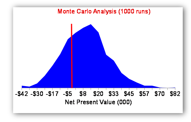
State legislative cost estimates. The Washington State Institute for Public Policy (WSIPP) is a non-partisan legislative research unit that has developed a method for prospectively estimating the costs and benefits of proposed legislative policies for the State. They use a benefit-cost framework for their analyses, to include estimates of impacts to society as a whole, including taxpayers, those individuals directly impacted by a policy, and other people in society indirectly impacted by a policy. WSIPP describes their research approach as follows. First, determine what works and what does not; what is efficient; what is the risk to the state in implementing individual policy options; and what interventions might be implemented together in a “portfolio” to achieve a common goal (WSIPP, 2012). WSIPP analysts begin by researching existing literature and meta-analyzing results to compute an effect size for a given intervention. Next, they examine costs and benefits from a societal perspective, considering the financial impacts on various parties in Washington State. The third step is a Monte Carlo sensitivity analysis of the estimated net benefits. WSIPP analysts present legislative decision makers with a graphical display of the likelihood that the net benefits of a policy will be greater than zero under a variety of assumptions. For example, Figure 1 displays the distribution of potential outcomes for a given policy option, demonstrating that, given the model assumptions employed, the likelihood of a positive net benefit from the policy (measured as net present value), is 75%.
41TFigure 1. 41TProbability distribution of the net present value for a policy intervention
In addition to these standard analytic frameworks for economic evaluation of preventive interventions, we review and consider models that depart from these standard approaches that have had some purchase in policy discussions of the financing of both clinical and community-based prevention. Several years ago, in the context of policy debates leading up to the passage of ACA, several organizations and consortia independently developed multiple-disease, multiple-intervention models to estimate the potential for reducing disease burden and health care (and in some cases other) costs through new investments in clinical and community-based preventive measures. Here we review the most prominent of these analyses: Milken Institute’s study, An Unhealthy America: The Economic Burden of Chronic Disease, Charting a New Course (DeVol et al., 2007); the Urban Institute’s return-on-investment model for Trust for America’s Health and the California Endowment (TFAH, 2008); and the prevention module of The Lewin Group’s analysis of the Commonwealth Fund’s health reform proposal (The Lewin Group, 2009). In addition, we discuss Archimedes, a simulation model that addresses clinical, administrative, and financial outcomes for a wide range of conditions with integrated physiology and care-process models (Schlessinger and Eddy, 2002).
Milken Institute. In an exercise to highlight the economic impact of increasing rates of chronic disease, the Milken Institute constructed a simulation model to project 20-year economic outcomes (2003-2023) for the U.S. population, both overall and for each state individually (DeVol, Bedroussian et al., 2007). The simulations are based on:
■ components that reflect demographic changes over the period;
■ a pooled cross-sectional analysis of the relationships between behavioral risk factors and seven specific chronic diseasesP2F[3]P; and
■ a model depicting a scenario in which preventive interventions result in lower rates of disease.
The simulation projects, for “baseline” and “optimistic” scenarios, the economic burden of chronic diseases in terms of direct medical care costs, indirect costs of lost workdays and lower employee productivity, and forgone national economic growth (measured as inflation-adjusted GDP) and intergenerational effects (measured as the educational attainment of the children of workers as a function of health and consequently income). The model does not take into account the costs of implementing any of the preventive strategies that are assumed to lead to lower rates of preventable chronic diseases.
The optimistic scenario includes assumptions of improved diet and physical activity, leading to reductions in obesity rates and consequently lower rates of several diseases; continued reductions in rates of smoking, lower rates of increase in air pollution, and improved early cancer detection through screening. A standard macroeconomic model simulates the impact of health on GDP, with life expectancy at age 65 serving as a proxy for health. The model assumes that health affects investments both in education and physical capital, with dynamic feedback between health and educational attainment over generations. Data on disease prevalence and costs of care are from the 2003 Medical Expenditure Panel Survey (MEPS), and other parameters on are based on data from the U.S. Census Bureau, the Behavioral Risk Factor Surveillance System (BRFSS), and the National Health Interview Survey (NHIS).
The model’s baseline simulation, assuming current trends continue, projects a 42 percent increase in cases of the seven chronic diseases by 2023, with an incremental cost of $4.2 trillion for medical care and lost economic output. The optimistic scenario, compared with the baseline scenario, would decrease treatment costs by $218 billion and decrease productivity losses by $905 billion, thus reducing the economic impact of disease by 27 percent, or $1.1 trillion in 2023. The model’s results are greatly dependent on the productivity component.
Days lost from work come from the NHIS, and are imputed to various chronic diseases. The value of each day lost from work was based on national estimates of GDP per employee. The costs of lost productivity while at work (presenteeism) were assumed to be 17 times as high as the costs due to absenteeism, based on a 2004 study by Goetzel and colleagues. Applying this large multiplier to days lost from work (for productivity losses due to presenteeism) and the use of the average wage rate per employee to calculate the value of lost productivity account for more than 80 percent of the estimated economic gains from preventing disease.
Urban Institute. In collaboration with the Prevention Institute, the New York Academy of Medicine, and with support from the California Endowment, the Urban Institute developed an economic model of the potential impact in the U.S. of primary prevention interventions at the community level to address nutrition, physical activity, and smoking (Levi et al., 2008; Ormand et al., 2011; Prevention Institute et al., 2007). The return-on-investment (RoI) model relied on a literature review of selected studies, 1975-2008, that reported on community-based public health programs aimed at improving health or changing behaviors affecting health.
Expensive diseases determined to be affected by these behaviors—diabetes, high blood pressure, kidney disease, stroke, heart disease, cancer, arthritis, and chronic obstructive pulmonary disease (COPD)—were grouped into three broad categories according to the time frames in which community interventions could be expected to have an impact. For uncomplicated diabetes and/or high blood pressure, an impact on disease prevalence and costs could be expected within 1-2 years; for the same conditions with complications (heart disease, kidney disease, and/or stroke), prevalence could be expected to be affected within 5 years; for selected cancers, arthritis, and COPD, public health interventions were assumed to reduce prevalence in 10-20 years. Based on the literature review results, prevalence rates for the short-term and 5-year disease groups were modeled as achieving a one-time reduction of 5 percent; rates for the conditions developing over the long term, cancer, arthritis and COPD, were assumed to be reduced by 2.5 percent. The intervention was assumed to be ongoing for the course of the model period. The authors did not assume any diminution from the effectiveness achieved in the first year and noted that they also did not build in additional positive impacts (reductions in disease rates) in years subsequent to the first.
The share of medical costs attributable to each of the diseases in the model was derived from a regression analysis of Medical Expenditure Panel Survey (MEPS), 2003-2005, so was limited to the population of non-institutionalized adults. Medical savings calculations were calculated as the product of the share of costs attributable to the three groupings of diseases (described above), total health care expenditures, and the assumed impact of community interventions on disease prevalence. The cost of the interventions was conservatively estimated at $10 per capita, across the entire population, based on reported costs in studies of community interventions that mostly ran from $3 to $8, and after consultation with experts about the $10 assumption. This represents marginal costs of the interventions only, however. The model also assumes a steady-state population, given disease prevalence for the included conditions as of 2004. It does not take account of any changes in mortality, or competing morbidity risks. Productivity impacts are not included in the analysis. At the national level, a $10 per capita expenditure on community prevention is estimated to save $2.8 billion in 1 to 2 years; $16.5 billion within 5 years, and $18 billion in 10 to 20 years, over what health expenditures for the affected diseases would otherwise have cost at 2004 prevalence rates.P3F[4]P The reported ROI is 2:1 in the short term and roughly 6:1 over both the medium and long term.
Unlike the Milken study, the Urban Institute model did not project forward current disease prevalence trends. However, it also focused exclusively on medical expenditure impacts, and projected increases in medical spending using CMS projections.
The Lewin Group “Path” proposal estimates. In 2009, The Lewin Group developed estimates of the cost impacts of provisions included in the Commonwealth Fund’s health reform proposal, “Path to a High-Performance Health Care System,” based on Lewin’s Health Benefits Simulation Model (HBSM) (The Lewin Group, 2009). The HBSM is a microsimulation model designed, in its baseline scenario, to represent the distribution of health insurance coverage and spending for a representative sample of U.S. households in 2010, using MEPS data 2002–2005. The data and model allow for estimates of coverage and spending under different coverage, payment, and benefits policies, for consumers, employers, state and local governments, and the federal government for 5-, 10- and 15-year periods.
The “Path” proposal included population health initiatives aimed at lowering rates of chronic and vaccine-preventable diseases. The model developed by Lewin estimated the health care cost impact of policies addressing tobacco use, obesity, alcohol abuse, and influenza immunization. The tobacco-related interventions included a federal cigarette (and other tobacco products) tax increase (to six times the current rate) and funding of smoking cessation programs with 10 percent of the new tax revenues. Assumptions about decline in use of tobacco reflected both the increased price due to the tax and the impact of cessation programs. Based on previous studies, health care costs were estimated to decline for former smokers for 15 years, with an increase in net health care spending due to longer lives after that period. Because the model produced estimates for the first 15 years post implementation (2010-2024), subsequent reductions in savings are not reported.
Obesity control measures include a one-cent tax per 12 oz. of sweetened soft drinks, with 10 percent of the revenues from the tax granted to states for obesity reduction programs, contingent on state enforcement of bans in the use of trans fats by restaurants and sweetened beverages in schools, and nutrition posting by chain restaurants. The model projected the national trend in the growth of obesity rates from 1998 to 2005 forward, used an estimate from the literature on the proportion of health expenditures due to obesity of 6.25 percent, and then assumed that the obesity control provisions would slow the growth of the share of national health expenditures attributable to obesity to one half the historic rate (from 0.4 to 0.2 percent). The “Path” proposal included a doubling of the federal excise tax on alcohol, and provided for a share of these revenues to be applied to national alcohol and illicit substance abuse prevention programs, and to block grants to states for similar purposes. The Lewin Group report cites the estimated economic burden of excessive alcohol consumption, but does not make any assumptions about the health or expenditure impact of reduced consumption due to the higher tax or increased programmatic activity to counter alcohol and substance abuse. Although a demand response to the higher purchase price of alcoholic beverages is not discussed, the estimated increase in federal revenues (which are just under half of reported excise take revenues of $9 billion annually) suggests that the modelers assumed that demand was relatively price-elastic. The modelers discussed the evidence about the cost-effectiveness of annual influenza immunization for different age groups but do not make an estimate of net impact on overall health spending. Finally, the results for separate provisions are adjusted for overlapping effects of various health plan provisions in the summary tables.
Archimedes. The Archimedes model is a highly detailed agent-based simulation model that uses available physiological and process-of-care data to predict clinical and economic effects of a wide variety of health interventions. Physiological variables are anatomical or biological, but also include risk factors such as age, blood pressure, and serum cholesterol. Process-of-care variables include service delivery, administrative, and financial factors. In the physiological component of Archimedes, an abnormal combination of variables constitutes a disease and clinical tests can be used to observe these variables at any point in time to indicate clinical events. To model health interventions, variables can be input as a value change or a rate of value change (Schlessinger and Eddy, 2002).
Mathematically, the physiological processes model consists of four equations: a natural projection of the variables and their interactions; the occurrence of events as a function of variables; the effect of interventions on events and variables; and the function of organs (Schlessinger and Eddy, 2002). The simulation of an agent over time uses differential equations and is a random process by assigning parameter distributions, derived from person-specific data. Any missing person-specific data is replaced with imaginary data that is consistent with real data, to accurately simulate the observed clinical events. If only aggregated data is available, it is translated into person-specific data by either using available data to model the relationship between the clinical event and an aggregated variable or making the simplifying assumption that a certain percentage of persons would experience the clinical event.
Prior to its application in predicting the impact of specific health interventions, the Archimedes model requires validation. Schlessinger and Eddy (2002) present several types of validation exercises that simulate clinical studies and compare them with the results in the observed study. In general, the equations must fit the data used to derive them; one or more of the equations must be accurate; and the prediction of health outcomes must be accurate. The authors consider a model valid if the equations are validated by at least one of the validation exercises. Once the model is validated, the level of model detail is verified based on three considerations: the scope of the question; the confidence of the model including all relevant clinical factors; and the availability of data.
The Archimedes model has been applied to diabetes. Eddy and Schlessinger (2003a, b) developed and then validated this application of Archimedes by building in information from clinical trials of different preventive interventions and comparing the model results to the real trial results. They found no statistically significant differences between model results and clinical trial results in most of their validation exercises; the correlation between the model and trial outcomes was r = 0.99.
Eddy and colleagues (2005) also employed the model in a CEA, comparing behavioral, pharmaceutical, and usual care to manage people at high risk for diabetes. The CEA used time horizons of 10, 20, and 30 years. Over 30 years and from the societal perspective, the intensive behavioral intervention for persons with impaired glucose tolerance was $62,600/QALY and for metformin therapy it was $35,400, in both cases compared to no intervention. An alternative model, developed by the Diabetes Prevention Program Research Group (DPPRG) and using the same interventions, produced different results, particularly for the behavioral intervention (Herman et al., 2005). Using a Markov model and a lifetime time horizon, the authors report a cost of $8,800/QALY for the lifestyle intervention, and a relatively similar $29,900/QALY for metformin therapy. In a commentary, one of the coauthors of the DPPRG study examines possible reasons for the different cost-effectiveness results, particularly as a number of clinically relevant results were similar (Engelgau, 2005). He concludes that different assumptions used in the two models about the rate of glycemic progression and the longer time horizon for the DPRRG model, which allows more complications to develop that could be offset by the intervention, are likely the major contributors to the differing results.
As alternative frameworks for the economic analysis of interventions to improve health emerged over the past half-century, so did different strategies for assigning value to different states of health. The first approach, cost-of-illness analysis, considered the direct costs incurred in medical care provided and the impact on human capital, the present value of productivity losses due to illness and premature death. Cost-effectiveness analysis (CEA) avoided the monetization of health outcomes by presenting the results of an analysis as the cost to achieve a single unit of a given health outcome, which could be either a health event such as a death averted, a case of cancer prevented, or a day of illness avoided; or a synthetic measure that could represent a combination of discrete health outcomes, such as a QALY. Benefit–cost analysis (BCA) requires that all benefits and costs be valued in monetary terms and non-market goods, including health and life itself, are valued according to the aggregate of individuals’ willingness to pay (WTP) for a given outcome. Different approaches to estimating WTP include capturing preferences revealed through market transactions and eliciting stated preferences. Each of these approaches is described below.
The choice of evaluating health impacts through CEA or BCA is largely determined by the decision about how health outcomes should be measured. In the U.S. in particular, and in economic analyses limited to the health services sector, CEA has been the approach overwhelmingly used. In multi-sector analyses, such as regulatory impact analysis, and in studies by international agencies such as OECD and WHO, BCA is much more likely to be used. The following subsections discuss the single-outcome (natural) and synthetic metrics used in CEAs, and the monetary valuation of health impacts in BCAs. Section 2.5 then compares and distinguishes the features of single-dimension metrics, HALYs, and WTP-based monetized measures. The final subsection addresses issues in the valuation of the benefits of prevention arising from federal estimation and budgeting rules and procedures.
Cases of illness or injuries, deaths, hospitalizations, and days lost from work or school are routinely collected health outcomes that often serve as a one-dimensional metric in CEAs of health interventions. The principle limitation of using single-outcome measures in CEA is that, the results of individual studies expressed in terms of different outcomes cannot be readily compared or combined.
Mortality measures are the oldest among population-based health status metrics. Preventable or premature deaths averted figured prominently in early regulatory risk assessments. Once CEA began to be used in health care studies, years of life saved, reflecting differences in remaining life expectancies, became a common metric.
HALY measures, which include QALYs, disability-adjusted life years (DALYs), and other constructs, represent the health-related quality of life (HRQL) impacts of different conditions, including functioning in domains such as mobility, emotion, social activity, and self-care. These measures assign index values to states of health that reflect particular states’ relative desirability or their implications for HRQL. The index values typically fall within a zero-to-one scale, where zero corresponds to death and one corresponds to perfect or optimal health. States of disability or morbidity have intermediate values, with lower values representing more severe impairments. For public policy decisions, the Panel on Cost-Effectiveness in Health and Medicine (PCEHM) recommends that these condition weights be based on the preferences of the general population (“community weights”), rather than those of patients or clinicians, to better reflect societal values (Gold et al., 1996).
Quality-adjusted life years (QALYs). Summary health measures for CEA were first suggested in the mid-1960s (Chiang, 1965; Fanshel and Bush, 1970). A decade later, theoretical arguments and analytical guidelines for using QALYs to evaluate health and medical practices were offered by Weinstein and Stason (1977), who noted that QALYs combine information about changes in survival and morbidity so as to reflect individuals’ willingness to trade off health and longevity. HRQL measures reflect both the nature of the health state—including, for example, observable and unobservable symptoms, functional capabilities, and individual perceptions of health—and the importance or value that individuals or populations ascribes to these various aspects of health. HRQL scales have been designed for specific disease or health conditions, but the most widely used metrics are based on generically described states of health, and thus are applicable across all diseases or conditions.
QALY metrics have been derived from both psychometrics (the theory and techniques of measuring psychological phenomena such as attitudes) and utility theory. Typically QALY metrics are constructed using a combination of psychological survey and decision-theoretical techniques. As preference-based measures, the values assigned to specific health states in an HRQL scale reflects the relative strength of preference for one state as compared with another.
The four most common methods for eliciting preferences for health states are: standard gamble (SG); time trade-off (TTO); category rating (CR) or visual analogue scale (VAS); and person trade-off (PTO).
■ In standard gamble, respondents must determine the conditions of equivalence between two alternatives, one of which is the certainty of being in the health state of interest (which is something less than full health). The other alternative has two possible outcomes: either full health or immediate death. The respondent is asked to name the risk of immediate death (with probability p), along with the complementary probability of living in full health (1-p) that would make this risky alternative equally attractive as the impaired health state. 1-p is then the value assigned to the impaired state of health.
■ In time trade-off, respondents are asked to choose between living in a state of impaired health for the remainder of life or living for a fixed (shorter) number of years in full health, followed by immediate death. The number of years in full health at which the respondent is indifferent between the alternatives is divided by remaining life expectancy to yield the value of the impaired health state.
■ In category rating or visual analogue scale, respondents are asked to rate a state of impaired health on a scale of 0 to 100, or mark a visual aid such as a “feeling thermometer.”
■ In person trade-off, respondents are asked to choose between health interventions and health states for others, indicating how many outcomes of one kind they consider equivalent in social value to a given number of outcomes of another kind.
These alternative methods ask different questions and can stress different facets of the relative value of various health states. Each of the four methods has distinctive advantages and proponents. Standard gamble is notable in that the choice embodies risk. Because most people are risk averse, weights for a given health state elicited through standard gamble tend to be higher (closer to optimal health) than weights derived from other elicitation methods. Economists advocate using standard gamble or time trade-off to elicit preferences because these approaches require making choices that reflect an opportunity cost, giving up one valuable good for another. Rating scale approaches like VAS are generally thought to be less burdensome for respondents than time trade-off or standard gamble, and result in fewer respondents opting out of the exercise. Some respondents refuse to engage in the exercise of trading off length of life or a higher risk of immediate death for a better health status (Brazier et al., 1999; Reed et al., 1993). Although standard gamble and time trade-off can be harder to administer (e.g., asking children with diabetes if they would be willing to live a shorter life to be disease free), these techniques allow for a more rigorous distinction between the annoyances and disruptions of a disease and substantial impacts that significantly reduce quality of life.
The person trade-off approach introduces other-directed or altruistic interests and has not been used as widely as the other approaches, although it was used to establish the original disability-adjusted life year (DALY) weights (Murray and Acharya, 1997). The person trade-off technique requires posing a large number of choices to construct a robust set of relative values for different diseases (Green, 2001). It has also performed poorly, relative to other approaches, in tests of reliability and internal consistency (Patrick et al., 1973; Ubel et al., 1996). Because the person trade-off technique requires posing a large number of choices to construct a robust set of relative values for different diseases, it is cognitively challenging, and has been found to be less reliable and less internally consistent than other approaches (Green, 2001; Ubel et al., 1996).
Disability-adjusted life years (DALYs). The World Health Organization (WHO) developed DALYs to serve as a summary measure of population health for the Global Burden of Disease study, launched in the mid-1990s (Murray and Acharya, 1997). The DALY measures potential years of life lost to premature death, adjusting those years to reflect the equivalent years of healthy life lost through poor health or disability. The DALY index scale inverts the QALY scale: for DALYs, 0 corresponds to perfect health and 1 to death. In contrast to QALYs, which reflect health states characterized generically, DALY values correspond to specific health conditions.
The approach taken to characterize and scale non-fatal health outcomes for DALYs has been revamped several times since the initial formulation of this measure for the 1990 Global Burden of Disease study (WHO, 2009: WHO et al., 2009). In the 1996 estimation of DALY weights, health professionals developed descriptions of particular disabilities and then other groups of health experts valued the disabilities, using the person trade-off method, as part of a deliberative process (Murray and Lopez, 1996; Gold et al., 2002). These DALY weights were constructed with two controversial features: higher weights given to years of adult productivity and decrements calculated from the worldwide maximum life expectancy (Japanese women). Neither feature is essential to the DALY calculation, and today DALYs have multiple formulations (de Hollander et al., 1999; Fox-Rushby and Hanson, 2001).
For the most recent GBD Study (2005), WHO is substantially revising the estimation of disability weights in response to criticisms of the DALY, including the measure’s exclusive reliance on expert panels and the use of the person trade-off method (Salomon, 2010; WHO, 2009;). The latest approach to developing disability weights includes a comprehensive re-estimation of about 230 unique “sequelae,” or states of health consequent to specific diseases and injury causes. This re-estimation includes both population-based household surveys in the U.S. and five other countries and overlapping open-access internet surveys, which will present simple paired-comparison questions to elicit respondents’ views of better and worse health states for about 50 of the sequelae. Using conjoint analytic techniques to infer cardinal weights for a population from individual rank orderings, this population-based information will be used by groups of health professionals to apply to the interpolation of values for all 230 sequelae, using ranking and VAS techniques. Finally, a third set of elicitation activities will be conducted with highly educated respondents at each of the original survey sites, using standard gamble and time trade-off techniques, to validate previous estimates of the disability weights (WHO, 2009).
Estimating a monetary value for a benefit that is not traded in the market, such as good health or a reduced risk of death within a certain time period, relies on the notion of individual WTP: the maximum amount of money an individual would exchange to obtain the benefit of good health or lower mortality risk, subject to the individual’s budget constraints.P4F[5]P Researchers can estimate monetary values for such nonmarket goods by asking people what they would be willing to pay for the health improvement or risk reduction. Specific methods for eliciting WTP within the general stated preference strategy include contingent valuation surveys and conjoint analysis.
WTP can be particularly helpful in coverage decisions for both private and public insurers. The insurers know what they would have to pay to cover the intervention. WTP provides a measure of what consumers would be willing to pay if they had to pay for the intervention out of their own pockets. If the benefit/utility is so low that consumers would not pay for it themselves, the likelihood that an insurer would cover it is greatly reduced.
A second broad strategy is to estimate WTP based on market information about related goods, referred to as revealed preference methods. One source of revealed preferences for estimating the value of health and mortality risk reductions is the compensating wage differential for riskier jobs, controlling for other factors that affect wage levels (wage-risk studies). Another source of revealed preferences for risk reductions is the voluntary purchase of safety equipment such as bicycle helmets by consumers. WTP estimates of the value of changes in the risk of premature mortality, using either or both stated and revealed preference studies, have been formulated as the value of a statistical life (VSL). VSL is a theoretical construct representing the aggregation over a large population of the value of reducing a relatively small risk of mortality. WTP for mortality risk reductions vary by the nature of the risk (e.g., whether the risk is undertaken voluntarily, such as sky diving, or is involuntary, such as from a plane crash) and the type of death (sudden versus prolonged, from cancer).
Many federal agencies use VSL in BCAs for regulatory impact analyses.P5F[6]P OMB guidance on VSL (Circular A-4, 2003) notes that various studies reported VSLs of between $1 million and $10 million; agencies may adopt their own estimate, as long as the rationale for the choice is given. Such rationales could include the concordance between the underlying WTP studies used and the nature of the risk addressed by the regulation at issue. The most recent research on VSL includes meta-analyses that variously reported mean VSLs of $2.6 million (Mrozek and Taylor, 2002), $5.4 million (Kochi et al., 2006), and $5.5−$7.6 million (Viscusi and Aldy, 2003), in either 1998 or 2000 dollars.P6F[7]P The Environmental Protection Agency (EPA), for example, uses a central estimate for VSL of $7.4 million (2006 dollars), and the Department of Transportation (DOT) of $6.0 million (2008 dollars) (DOT, 2009; EPA, 2010).
Although much of the effort of calculating HALYs involves establishing the relative values of different states of health rather than changes in longevity, survival impacts usually overwhelm HRQL impacts in CEAs using QALYs. Chapman and colleagues (2004) reviewed 63 studies with a total of 173 paired cost-effectiveness-ratios, reporting both cost per life year ($/LY) and cost per quality-adjusted life year ($/QALY), The authors reported that quality adjusting life years resulted in a relatively small difference between LY and QALY ratios, with a median difference of $1,300. A separate review by Tengs (2004) of 110 cancer prevention, early detection, and treatment interventions, also examined differences between $/LY and $/QALY ratios, with findings consistent with those of the Chapman study: the LY and QALY ratios had a very high rank order correlation. The conclusion of both studies was that quality-adjusting life years would have affected decisions about cost-effectiveness for only a small fraction of the studies—8 and 5 percent in the Chapman and Tengs studies, respectively—if $50,000 per life year or QALY were used as the decision threshold.
Constructing a HRQL index and a HALY metric that reflects the general population’s relative assessment of different health outcomes involves surveys similar to those to elicit WTP. By design, however, HALY measures are independent of individuals’ income or wealth, while WTP surveys capture differences among individuals that reflect different resource constraints. In practice, however, the income or wealth term is not always statistically significant in WTP studies and HALY measures may be influenced by individuals’ income or wealth.P8F[9]P Another important distinction is that WTP values demonstrate the extent of tradeoffs that individuals are willing to make between widely different uses of resources, whereas HALY metrics limit trade-offs to those between different states of health. Finally, even though HALY measures are based on surveys eliciting individual choices, some welfare economists argue that these choices do not fully conform to the theoretical concept of utility (Dolan and Edlin, 2002).P9F[10]
Using a cost-per-QALY dollar limit as a general guide when using CEA to allocate resources or to establish a threshold for policy action has been hotly debated, and even agencies such as the National Health Service in Great Britain, where CEA is considered in funding decisions for new services, deny the existence of an explicit cutoff.P10F[11]P It can be argued that using such a threshold value essentially turns CEA into BCA (Phelps and Mushlin, 1991). A wide range of QALY threshold values have been proposed or suggested as implicit in policies adopted in the U.S., from $50,000 to $297,000 per QALY, and even higher if fully inflated to current dollars (Braithwaite et al., 2008; CDC, 2011a; Hirth et al., 2000 ).
2.6 Additional issues related to valuing health impacts: Time horizons and rules governing federal budgeting and projections
Unfortunately modeling methodologies developed to maximize the rigor in the clinical or epidemiological context are sometimes not as helpful in informing public policy decisions. The federal government has developed specific rules and methodologies to help policymakers make informed decisions between competing policy priorities. These competing priorities range well outside health and health care and include such disparate issue areas as defense spending, tax policy and government procurement. A prime example is the way the Congressional Budget Office (CBO) models expected spending on current and new federal programs. A parallel process has evolved in the executive branch, with the exceptions of two long term entitlements, Social Security and Medicare.
The opposite is also true; the modeling conventions of public agencies, which are designed to maximize ease of comparison across policy options, are sometimes not helpful in informing public policy decisions on health issues that do not have the same dynamics as the typical policy choices. For example, chronic diseases can take decades to manifest and prevention interventions consequently take decades to generate savings. While the modeling conventions of organizations like CBO and CMS’s Office of the Actuary work well to help congressional and administration decision makers choose between most policy options, often they do not capture the natural history of a chronic disease, changes in quality of life, or spending and savings beyond the first ten years.
Both the legislative and executive branches typically use a ten-year budget “window” for policy projections. Exceptions include the supplemental 75-year projections done for the Social Security and Medicare Trustees’ Report, and CBO’s annual Long Term Budget Outlook report. (Also, as discussed earlier, CBO’s practices are changing and projections are sometimes made for longer time horizons.) The 10-year budget window, originally 5 years, evolved over time for two reasons. First, modeling capabilities had improved to the point that there was confidence the projection period could be expanded with meaningful results. Second, enterprising congressional committee chairs were increasingly moving spending into the sixth and seventh year of their proposed programs. The second conventional practice of public sector modelers, using nominal dollars rather than dollars discounted either for inflation or the time value of money, reflects the idea that the estimate should present actual out-year spending, not some form of discounted out-year spending. Notably, CBO’s 25- and 75-year Long Term Budget Outlook projections report spending as a percentage of GDP. In the context of prevention, a short projection period is problematic. Many current prevention activities target behavior that will not have a serious health consequence for years to come. As we saw with the other modeling methodologies, lifetime or at least 25-year estimates are more common. As we know from the natural histories of the disease we are trying to prevent, an obese person does not develop type 2 diabetes in the year after putting on weight and the person diagnosed with diabetes does not begin to experience the full onslaught of complications in the next 5 years.
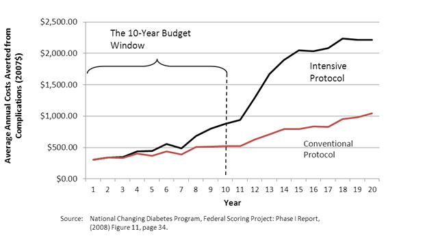
Figure 2 illustrates this problem, using the example of type 2 diabetes. The figure shows the spending averted on diabetes and diabetes-related complications for two cohorts, one with intensive control of their glucose levels and one with more conventional control. The intensive control cohort experiences the type of management typically found in state-of-the art diabetes disease management programs. The figure demonstrates that intensive control reduces future diabetes spending, but that those reductions do not begin until about the eighth year of the intervention, with the vast majority of the savings occurring after the first ten years. Clearly the 20-year window used here gives a more complete picture of the effects of the intervention.
41TFigure 2. 41TThe Budget Window and Disease Progression—Type 2 Diabetes and
Glucose Control Efforts: Average Annual Costs Averted from Complications
If CBO were to expand its usual 10-year budget window, at least for cases where a longer perspective is needed to give policymakers a more accurate picture of the tradeoffs, it would then trigger renewed debate over the use of nominal dollars. The current use of nominal dollars is less of a problem over ten years than it would be over a 25-year period or over the lifetime of the patient. The concern is that nominal dollars ignore both the effects of inflation on out-year spending and the time value of money.
CBO has confronted this dilemma in the past and will increasingly confront it in the future, especially with regard to preventive services and chronic disease interventions. For example, as far back as the mid-1980s when CBO had to estimate the budgetary impact of a reformed federal employee pension system, they present two sets of estimates: one set with their traditional budget window in nominal dollars and another set of actuarial estimates using lifetime present value methodology. The first estimate was consider the official score, but the set estimate provided decision makers with a more comprehensive analysis of the budgetary impact, if they decided to pass the reform legislation. In this example the concern was in the opposite direction, i.e., new pension systems tend to significant savings in the early years matched by significant spending in the later years once workers begin to retire.
Section 3. Modeling the Impacts of Investments in Prevention: Estimation Methods
Estimates of the cost of illness or simulations of the economic value of health interventions are often subjected to scrutiny by a variety of stakeholders of the health policy under evaluation. In the early decades of economic evaluation of health interventions (1960s through the mid-1990s), few standards existed to guide the development of studies; studies employed widely divergent assumptions for key model decisions. Over time, health economic methods have grown increasingly standardized. Both journal reviewers and outside consumers of health economic studies have come to demand substantial transparency and standardization in core modeling decisions and the presentation of core results from these studies. Recent models build upon epidemiological and clinical research conducted over the prior two decades that have attempted to establish the efficacy of particular interventions in both clinical and community settings.
Understanding the basic methodological standards and best practices that are commonly accepted in the prevention modeling field will assist policy makers in their assessments of new health economic information as it is presented to them. In section 3.1, we first review the general estimation choices and steps that are taken in prevention modeling studies, the importance of each step, and the opportunity to introduce bias associated with each choice or step. Next, in section 3.2, we discuss different estimation or modeling approaches and discuss their relative strengths and weaknesses in terms of modeling effort and flexibility. After discussing the basic modeling framework and the steps taken to produce estimates, in section 3.3 we discuss alternative approaches to measuring outcomes and assessing economic impacts and potential new directions in valuing health states that policy makers may wish to encourage. In section 3.4, we discuss the underlying principals and rationale for using the results of economic models of preventive interventions, namely to assist in making difficult decisions under conditions of uncertainty.
This section reviews the initial study design choices that shape cost-effectiveness analyses and then reviews options involved for performing sensitivity analyses.
Estimation and standards of the baseline analysis. The initial design of a cost-effectiveness study involves a set of choices that will shape the results that flow from the analyses. These choices include how outcomes will be measured, the selection of a comparator, a specification of the time horizon, the extent to which future costs and benefits will be discounted to reflect their present value, and the perspective of the study which will determine which types of costs and benefits will be included in the analysis.
The comparator. The cost-effectiveness of an intervention or new technology is a relative estimate which depends upon the scenario to which it is compared. A comparator (also known as the baseline or status quo) scenario is the counterfactual alternative situation whose costs and benefits are compared to the intervention or policy choice scenario in order to determine cost-effectiveness. In a cost-effectiveness analysis, a model is used to simulate the costs and benefits of intervention strategy and the comparator counterfactual situation, and then the incremental differences in costs and benefits are used to calculate the incremental cost effectiveness ratio (ICER). The equation for the ICER is written as:
(CostRInterventionR – CostRComparatorR) / (BenefitsRInterventionR – BenefitsRComparatorR) … (3.1.1)
Note the importance of the comparator in determining the size of difference in costs and benefits and driving the ICER. Because of this, policy makers should be certain to consider whether the comparator scenario or scenarios used in the analysis appropriately fit the policy context to which the results will be applied.
While many older studies utilized a no intervention scenario as their comparator, a more realistic comparator is some form of estimate of the services the model’s target population would be expected to use in the absence of an intervention. For example, in a recent paper evaluating the cost-effectiveness of dilated fundus examinations of persons newly enrolling in Medicare at age 65, the authors compared the intervention scenario to a comparator of usual care, where usual care was the estimated annual probability of a dilated fundus examination of current Medicare recipients (Rein et al., 2012).
Time horizon. The time horizon refers to the number of years the cost-effectiveness model is run after model initiation. The time horizon is important because it defines the scope of benefits and costs that will be included in the model. Longer time horizons are able to capture more of the true costs and benefits of the intervention. In practice benefits and costs that occur far in the future are more speculative and often rely on model-generated estimates of disease impacts that are less certain than clinical observations or trial data. The appropriate time horizon will depend on the relevant decisions being made by the policy maker. A study that employs a lifetime time horizon is well within the bounds of acceptable and sound research practice. However, a lifetime time horizon may not provide suitable information when a policy maker is most concerned with costs and benefits that accrue over the short or intermediate term. Simulation results have demonstrated that the specification of the time horizon can have substantial impacts on the cost-effectiveness results generated from a model, especially when the model employs the standard 3 percent discount rate (see next section) (Sondhi, 2005).
The discount rate. The discount rate represents the time preference of the model for benefits that occur today in comparison to benefits that occur in the future. A foundational concept of classical microeconomics is that individuals prefer benefits gained today over identical benefits gained in the future and that the extent of this preference can be estimated based on a rate function (Menger, 1892). Put simply, individuals prefer $1 today than $1 next year and the degree of this preference can be measured by the percentage of that $1 that would have to be paid to convince someone to exchange the $1 today for the $1 next year. The value of future benefits after accounting for discounting is called its net present value (NPV) and is calculated as:
NPV = ValueRfutureR / (1+r)PnP … (3.1.2)
Where Value Rfuture Ris equal to the value of the specific benefit or cost at the time it occurs in the future, r is equal to the discount rate, and n is the number of years in the future that the benefit or cost occurred.
The discount rate is sometimes confused with the inflation rate, but this is incorrect. The discount rate measures true differences in value attributed to current benefits as compared to those that occur in the future, whereas inflation measures only the erosion of purchasing power of a currency over time. The discount rate is applicable even in a world where inflation is equal to zero; the vast majority of cost-effectiveness models do in fact constrain inflation to zero (Haddix et al., 2003).
Discount rates used in cost-effectiveness studies are highly variable across studies, but generally range from 0 to 10 percent (Nixon et al., 2000). The PCEHM reviewed a wide range of standards used in the United States to set discount rates before specifying 3 percent, an approximation of the average shadow price of capital over the long term in the United States, for use in its recommended reference case analysis. (Gold et al., 1996).P11F[12]P This standard has been widely adopted in United States cost-effectiveness research.
The discount rate determines the extent to which benefits that occur across the time-horizon influence the policy decision made based on the model’s results. Figure 3 illustrates the number of years at which the present value of $1 of future benefits or costs falls to $0.50, or half its original value. As the figure illustrates, the value of future benefits and costs falls rapidly with an increasing discount rate. At a rate of 1 percent future benefits and costs maintain over half their value until 70 years after the simulation begins. In contrast, at the most commonly used discount rate of 3 percent, future benefits and costs retain over half their until 24 years after the simulation begins, a value that falls to 14 years at a rate of 5 percent and to 7 years at a rate of 10 percent.
41TFigure 3. 41TYear at which the Present Value of a Future Benefit or Cost is Worth Approximately Half Its Future Value
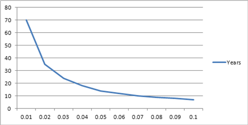
Researchers sometimes argue that the time-horizon chosen is irrelevant because most future benefits are heavily discounted in terms of their present value. As figure 3 illustrates, this can be a potentially error-inducing generalization. At the 3 percent discount rate, the one most commonly used by modelers in the United States, future benefits and costs still hold substantial present value even when they occur decades into the simulation. Policy makers who are substantially more concerned with the near term costs and benefits of an intervention should seek out results that utilize higher discount rates in their analyses.
Study Perspective. The study perspective refers to the person, individual, or population to which the costs and benefits of an intervention are realized. For example, the costs and benefits of an intervention are different from the perspective of an individual than from the perspective of a health plan. The individual generally pays only a small portion of the costs of health care and receives all the health benefits. In contrast health plans may pay virtually all the costs of the same intervention, but may not enjoy any of the benefits of the preventive health affects occur after the patient transfers to a different health plan. Mapping costs and benefits from different perspectives allow the model results to illustrate differences in incentives across stakeholders involved in the intervention.
Perspectives taken in cost-effectiveness models include the patient, provider, hospital, health plan, health care system, and the societal. In some circumstances, it may not be beneficial for a study’s authors to present all perspectives. The PCEHM present the example of a hypothetical medical device that is cost-effective or cost-saving from the hospital’s perspective, but achieved this success by transferring costs to other aspects of the health care system (Gold et al., 1996). To facilitate comparisons across studies, and to avoid cherry picking of favorable perspectives, current cost-effectiveness standards recommend the inclusion of the a societal (or health care if societal is not feasible) perspective as a reference case, even if the primary interest of the paper is to examine differences in cost-effectiveness at a more granular level.
Model Validation. In scientific practice, validation refers to the ability of an experiment or scientific inquiry to uncover true causal relationships, and the extent to which the relationships in the study can be extended to other situations. In the world of prevention modeling, researchers construct mathematical representations of reality in order to test the impact of changes in policy or treatment. The key questions of validity regard whether the results generated by the model can be used to make policy decisions.
Preventive services models are often evaluated in terms of their fidelity, and their internal, cross-model, and external validity. Fidelity, also known as face validity, refers to the integrity of the model structure the quality of the data used to populate it, and the degree to which a model adheres to reality (Feinstein and Cannon, 2001). Models should be constructed based on current medical understanding of the disease or phenomena under consideration. Although models must always simplify reality in order to be tractable, models that omit important aspects of disease progression that affect either patient outcomes or costs lack validity in making economic decisions.
In experimental design, internal validity refers to the quality of evidence that results from a particular experiment. Selection bias or other forms of confounders weaken the power of evidence obtained from a trial. In theory, simulation models avoid selection bias and confounders because simulated agents can be matched perfectly in terms of their traits. In practice, bias can be introduced by the modeler either through conscious or inadvertent parameter selection that favors a certain policy of choice, or through the use of low-quality data or studies to populate the model’s parameters. The threat of bias can be diminished by publishing the model’s parameters and sources and through a review of those parameters by independent experts.
Another test of the internal validity is to assess whether the model can recreate the epidemiological data used to program it. When the population parameters of a model are specified to fit the epidemiological context of its input data, a model should be able to recreate the population prevalence and/or incidence seen in that study. Failure to do so can indicate an internal programming error, the incorrect logic applied to the use of a given parameter, or a confounding dependency embedded in the model’s processes.
41TTable 141T41T.41T Threats to Model Validity by Type, their Importance, and Methods of Detection and/or Amelioration
| Type of Threat | Importance | Methods of Detection and/or Amelioration |
| Threats to Fidelity |
|
|
| Programming errors | High | ■ Systematically vary model parameters to extreme values to identify model processes causing errors. ■ Budget appropriate time for model testing and debugging. ■ Utilize personnel with programming expertise. |
| Unrealistic, inaccurate, or overly-simplified disease natural history model | Very High | ■ Solicit clinical and other subject matter expertise to review model structure and assumptions. ■ Focus on natural history changes that result in a change of symptoms or costs. Stages that do not directly influence a change of symptoms or costs can be combined with other stages. |
| Threats to Internal Validity |
|
|
| Systematic bias in selection of parameters | Very High | ■ Solicit expert review of parameters. ■ Be alert for omission of important studies. ■ If systematic bias is identified, heavily discount results. |
| Use of low-quality data as the result of lack of information | Low | ■ Solicit expert review of parameters. ■ It is not uncommon to have weak data sources for some model parameters. Well-designed studies will include sensitivity analyses that test the impact of weakly measured parameters. |
| Model does not recreate data used to program it | Moderate | ■ Evaluate information comparing the model’s epidemiological inputs to the comparable estimates created by the model. ■ Consider causal relationships in the model, it is possible that the correct parameter value is being misinterpreted or used incorrectly. ■ Model calibration can improve the model’s internal predictive performance. |
| Poor cross-model validation. Model does not produce similar results to other simulation models. | Moderate to Very High | ■ Evaluate reasons why the models predictions would differ such as whether model uses different input data, or whether the model uses different disease natural history assumptions. ■ If different, evaluate if different data or model formulation is a suitable alternative to existing models. |
| Threats to External Validity |
|
|
| Model does not predict out of sample epidemiological data | Moderate | ■ Adjust model’s confounding parameters to match external data set. ■ Consider if differences are reasonable given uncertainty in model’s epidemiological parameters. ■ Calibrate model if differences are extreme. |
| Model utilization rates do not match community estimates utilization rates | Low | ■ Assess the degree to and manner in which community utilization rates influence the model’s results. ■ Consider whether the utilization rates used in the model are logical and internally consistent across utilization, effectiveness, and costs. ■ Assess how model results apply to settings in which community rates of service utilization differ. |
Cross-model validity refers to the ability of a simulation model to produce estimates that are concordant with those published earlier using similar models (Eddy et al., n.d.). If a model uses the same basic data and structure as earlier models, then it should result in epidemiologically similar estimates. If it fails to do so, then its internal validity should be questioned, as the same data is resulting in different results. Differences in estimates can occur from the application of the model to a different context, through differences in model specification, or from the incorporation of new or different data inputs. The purpose of cross-model validation is to articulate how estimates generated from a given model are similar to or differ from earlier modeled estimates regarding the same topic. Caution should be used in rejecting model estimates simply because they do not conform to earlier estimates, especially when only one previous estimate exists or when all previous models were generated by the same author or team.
External validity refers to the ability to generalize results obtained by the model to a wider set of circumstances. In most simulation contexts, external validity would refer to the ability to make decisions about the actual world based on the findings of the model. Because simulation models are always simplifications of complex systems that in themselves occur with some degree of random variation, models will rarely result in exact reproductions of empirical reality. The topic of the external validity of simulation results is quite wide and encompasses many areas of philosophy of science. Questions of how close a model’s predictions must be to an externally generated dataset in order to be considered valid are in fact impossible to answer. Philosophers such as Popper, Kuhn, and Feyerabend have argued that similarity cannot be judged in absolute terms but instead must be understood relative to the situation (Feinstein and Cannon, 2001).
In practice, what this means is that the external validity of a model is often judged by comparing model results to external data, articulating the degree to which the model recreates important outcomes of interest, and allowing the reader to decide upon the level of external validity the model possesses. Often this exercise is quite difficult, as appropriate external data for validation purposes may not be available or may not have been collected for a population that is similar to the one of interest in the simulation model. In limited circumstances contests have even been sponsored to test the external validity of several different models developed by different research teams (Fourth Mount Hood Meeting Report, 2007). Policy makers evaluation a model’s external validity should consider whether the authors attempted to compare their model to external data, the circumstances which might have limited these comparisons, the extent to which these comparisons were documented in technical appendixes, the differences between the modeled data and the external data, the degree to which these differences might influence the model’s results, and whether areas of model weakness were appropriately accounted for in sensitivity analyses.
Modeling uncertainty. Estimates derived from prevention models contain uncertainty from at least three sources. Individual random variation is referred to as first-order variability, and usually occurs in agent-based models that allow for individual differentiation within cohorts. First-order variability is not a primary concern in most prevention models.
Variability in the measurement of parameters is referred to as second-order variability and is a primary concern in all models. Second-order variability refers to the fact that the parameters used in a model are sample estimates. In the best of circumstances these parameters have been drawn from experimental studies and will have been measured with error. In many other circumstances, parameters may be based on averages of estimates across studies, on expert opinion, or simply upon assumptions. Models should attempt to account for the uncertainty caused by their parameters through univariate and probabilistic sensitivity analyses (described below).
Structural uncertainty refers to embedded assumptions of the model process that may be incorrect. For example, a model may assume a linear relationship between disease progression and time, when in fact this relationship is nonlinear (McKay et al., 1999). Other aspects of model uncertainty may include the options of treatment offered to patients after diagnosis. For example, in a paper on the cost-effectiveness of glaucoma treatment in the developing world, the authors developed estimates based on an assumption of a one-time laser surgical intervention following diagnosis and assumed no option for pharmaceutical treatment for diagnosed patients (Wittenborn and Rein, 2011). In practice structural or model uncertainty is rarely addressed outside of somewhat ad-hoc scenario testing of alternative outcomes. Policy makers concerned with structural uncertainty may wish to consult work on Bayesian simulation approaches to the problem (Briggs, 2000).
Univariate sensitivity analyses. Univariate sensitivity analyses offer a common approach to testing variation in a single parameter. In univariate sensitivity analyses, a parameter’s value is varied to the extremes of its plausible ranges while holding constant other variables in the model, in order to assess the impact of that single variable on the model’s results. Univariate sensitivity analyses are quite valuable in identifying the parameters to which the model is most sensitive.
Often the results of multiple univariate sensitivity analyses are arranged in a tornado diagram, listing the most influential variable in terms of its impact on the ICER at the top to the least influential variable tested at the bottom. For example, Figure 4 illustrates the univariate sensitivity of a new screening strategy for hepatitis C to one-at-a-time changes in model parameters.
41TFigure 4.41T Example of a Tornado Diagram: Univariate Sensitivity of the Incremental Cost-Effectiveness Ratio of Birth Cohort Screening with Standard Treatment Compared to Risk based Screening Assuming Pegylated Interferon with Ribavirin Treatment to Changes in Key Model Parameters
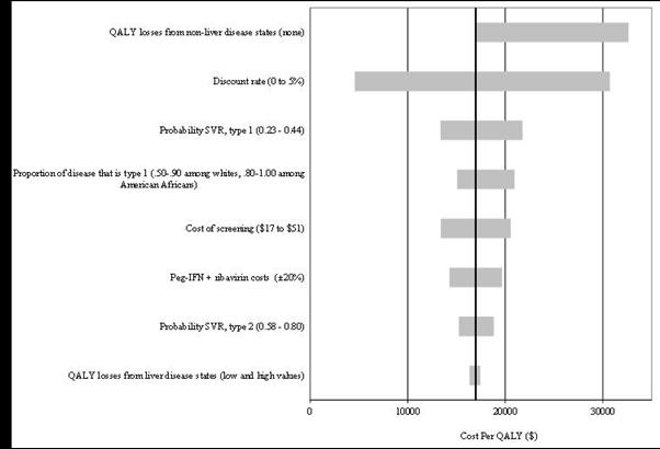
Note: Standard treatment = pegylated interferon with ribavirin; QALY = quality-adjusted life year; SVR = sustained viral response; PegIFN = pegylated interferon with ribavirin
Adapted from: Rein, Smith, and Wittenborn, et al (Forthcoming) The Cost-effectiveness of birth-cohort screening for hepatitis C antibody in U.S. primary care settings. Annals of Internal Medicine.
Policy makers should evaluate which parameters were selected for inclusion in the univariate sensitivity analysis and the range of the values considered in the analysis. Major weaknesses of the model can be hidden through omitting key parameters from such analyses and results can be made to look either more or less certain based on the ranges chosen. The ranges should be logical, justifiable, and when possible based on empirical observations.
Probabilistic sensitivity analysis and credible intervals. Probabilistic sensitivity analysis (PSA) is a simulation process to measure the impact of uncertainty across all the major parameters in the model (or at least a set of major parameters). To conduct a PSA, the researcher specifies the distributional shape and parameters for each of the variables in the model. Ideally, these parameters should be drawn from empirical data measuring the standard error of the parameter and common distributional assumptions specified to the parameter of interest (Briggs et al., 2006). In the event the parameter variance cannot be derived empirically, the modeler may construct it from the range of available estimates, to match expert opinion, or using published guidelines (Doubilet et al., 1985).
The modeler then creates an n x k matrix of parameter values where n is the number of simulations to be run and k is the number of parameters to be varied in the PSA. Each parameter is then sampled from its target distribution n times to create a matrix of input values for use in the simulations. This table of possible input variables is then used to run the simulation so that each iteration represents the model results given that particular draw of parameter. PSA results can then be evaluated to estimate the mean and the credible interval of the simulated results, or to plot the entire distribution of the simulated results.
The ability to create credible intervals, the Bayesian alternative to confidence intervals, is one of the key advantages of conducting a PSA. In concrete terms, using the simulated results we are able to create the possible range of outcomes predicted by the model after propagating parameter uncertainty through the entire model structure.
Cost-effectiveness acceptability curves. Policy makers should realize that all prevention models are uncertain; their results are probabilistic, not deterministic. (This is true, although not obvious, even when model analyses have not been conducted in a probabilistic manner). Thus assessments of cost-effectiveness can only be stated as probabilities, not certainties, and are contingent upon the amount a policy maker is willing to pay for given preventive benefit.
The results from probabilistic sensitivity analyses can be used to create cost-effectiveness acceptability curves (CEAC), which summarize the probability that each scenario under consideration is the most cost effective given different values of willingness to pay (WTP) for the benefit. CEACs are constructed by comparing the net health benefit of each intervention, for every simulated iteration, at each value of willingness to pay. The net benefit is equal to:
Net BenefitRiR = BenefitRiR ∙ WTP – CostRiR … (3.1.3)
Where i indicates the scenario measured, and WTP indicates the particular willingness to pay valuation used. Because net benefit is linear, net benefit estimates for each scenario can be directly compared without having to rely on incremental results. To create a CEAC, the research compares the net benefit of each scenario at each WTP value and codes the intervention with the largest net benefit the most cost-effective. The researcher then calculates the proportion of simulations “won” by each intervention at each WTP value and charts these proportions against WTP in a line graph.
For example, Figure 5 displays the probability that each of four screening options is the most cost-effective given a range of WTP values per incremental QALY gained (Rein et al., forthcoming). The far left of the figure represents a policy maker who is willing to pay nothing per incremental QALY gained. At that value (WTP=$0), 100 percent of this model’s simulations determined that no screening was the most cost-effective alternative. Progressing rightward on the x axis, the WTP increases and the probability that no screening is most cost-effective decreases. At a WTP value of $16,000 per QALY saved, birth-cohort screening with standard treatment becomes the option most likely to be cost-effective. The probability that birth-cohort screening with standard treatment is most-cost-effective increases to near certainty at a WTP value of approximately $27,000 per QALY gained and then begins to fall as birth-cohort screening with more expensive direct acting antiviral therapy becomes more likely to be most cost-effective at higher values of WTP. Note that risk-based screening, the current standard of care, is never the most likely to be the most cost-effective.
41TFigure 5. 41TExample of Cost-effectiveness Acceptability Curve (CEAC). The Cost-effectiveness of Four Possible Screening Alternatives for Hepatitis C
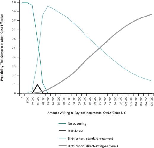
Adapted from: Rein, Smith, and Wittenborn, et al, 2012. The cost-effectiveness of birth-cohort screening for hepatitis C antibody in U.S. primary care settings. Annals of Internal Medicine.
CEACs have limitations in assisting decision makers (Koerkamp et al., 2007). The primary disadvantage of CEACs is that they ignore extreme outcomes. For example, CEACs only detects the proportion of scenarios in which a scenario “wins” and ignores information about when that scenario loses. As a result, a scenario with a lower expected value may appear to be more cost-effective than a scenario with a higher expected value if it is more frequently cost-effective but the instances in which it is not lead to extreme losses. Related to this concept, while CEACs present the probability of making a wrong decision, they do not provide any information about the consequences of that decision. In addition, CEACs may create urgency for policy action when an intervention appears highly likely to be the most cost-effective, even though the net benefits of this intervention may be small. For these reasons and others, alternatives to CEACs such as credible intervals and value-of-information analysis are important for understanding the uncertainty surrounding a decision.
Value-of-information analyses. Value-of-information (VOI) analyses quantify the potential opportunity losses that can result from making an incorrect decision between mutually exclusive policy options. Choosing between policy options always entails a degree of uncertainty and a consequent probability of an incorrect decision. VOI analyses build off simulation results to estimate the dollar value of additional research on a topic with the aim of reducing uncertainty. VOI analyses can help set priorities for additional research by identifying which decisions could result in the greatest opportunity losses if made incorrectly and by identifying the value of additional information gained about specific parameters used to make those decisions.
The value of information, or expected value of perfect information (EVPI), is a function of the incremental cost-effectiveness of a specific technology of interest, the level of uncertainty surrounding the cost-effectiveness estimate, and value applied to the benefits gained by the intervention (Briggs et al., 2006). Although benefits are often measured in QALYs saved, VOI approaches can be applied to any concrete benefit that a policy is designed to maximize.
EVPI can be estimated numerically or non-parametrically from simulation results. Numerical approaches are easily implemented but depend upon assumptions that may often be violated by results generated from decision-analytic approaches. For example, if one assumes that the incremental net benefit (INB) of an intervention is normally distributed, then the EVPI of an intervention can be solved as a function of the slope of the loss function, the estimated INB, and its variance. Unfortunately, INB can rarely be assumed to be normally distributed as most decision analytic models combine parameters from different experimental observations with a range of distributions. Alternatives to numeric approaches include sampling algorithms from simulation results, as well as minimal modeling, and meta-modeling techniques which attempt to replace the decision analytic model with a statistical alternative (Meltzer et al., 2011; Tappenden et al., 2004).
Decision models can take many forms, from simple spreadsheet analyses and decision trees to more complex model formulations. Policy makers may sometimes request specific model frameworks, given past familiarity, or because they have observed presentations by strong modelers that showcase certain techniques. Prescribing the modeling technique to be used (for example in a request for proposals) is likely not advantageous as every modeling approach has distinctive advantages and disadvantages compared to others. When choosing a model, the researcher should consider at least the project budget and timeline, the immediate use and future reuses of the model, and the minimum degree of complexity needed to model the problem correctly. Adding model complexity may increase model precision, but it does so at the cost of time, research dollars, and model transparency.
In this section we first discuss generic types of models, and then consider some common alternative modeling structures, their strengths and weaknesses, and their ideal applications. The purpose of the section is to inform policy makers about different modeling options so that they can understand the implications of different modeling choices.
Model Types. Several different model types can be employed across a variety of model structures. Kim and colleagues (2008) classify models in terms of four distinct dimensions: (1) the ability of individuals in the model to interact (static versus dynamic); (2) the ability of new individuals to enter the model as the time steps of the model progresses (open versus closed); (3) whether population averages are used or the model tracks individual actions (aggregate versus individual-based); and (4) whether model transitions are variable or fixed (stochastic versus deterministic).
Static models use fixed parameters that are constant throughout the life of the model. Dynamic models allow changes between states in a model, usually dictated by disease incidence parameters in a static model, to depend upon both fixed parameters (such as the force of infection, and the rate at which people contact each other) and changing or dynamic values such the proportion of individuals that are infectious or susceptible to infection. Because of the complexity of developing dynamic models, static models are more frequently used and likely preferable, except in circumstances where the intervention is likely to affect the transmission of disease. For example, Bauch and colleagues (2007) developed a dynamic model of hepatitis A transmission to estimate the cost-effectiveness of universal vaccination in Canada. The dynamic form of the model was able to capture additional herd immunity benefits of vaccination to unvaccinated individuals.
A model’s openness refers to its ability to incorporate new populations over time. Open models allow new populations to age-in as older population die out. This feature is particularly important in disease transmission models where new susceptible populations may join the model as the original susceptible population is depleted. Alternative versions of an open model may allow new cohorts to be created to enroll in an intervention in time steps subsequent to the model’s initiation. As with dynamic models, open models are more important for disease transmission models than for models of chronic diseases where disease acquisition of one individual does not depend on the status of other individuals.
Aggregate models refer to models estimated at the population level. Examples of aggregate-level models are decision-tree and some state-transition models (see below), where the model estimates are created from multiplying transition probabilities times the proportion of the population in a given state. In contrast, microsimulations and agent-based models (see below) are examples of individual-level models. As their name implies, individual-level models estimate the model’s processes at the level of an individual agent. These agents have both memory and embedded decision rules that govern their behavior. Aggregate-level models have the advantage of producing cleaner estimates and are easier to program and manage. Individual-level models may offer some advantages in modeling group interactions, and can also be used to ease the modeling of very complex systems.
Fixed versus stochastic parameters refers to the element of random chance in the instantiation of model events. In general, models at the aggregate level use fixed parameters, while microsimulations and agent-based models use stochastic parameters. Person-level variation results in a much greater degree of variation in the model’s estimates. Although methods exist to adjust the credible intervals of net benefits derived from stochastic models, the higher variance of estimates inherent to individual-level models remains one of their chief limitations (O’Hagan et al., 2007).
Decision-tree models. Decision trees are model structures that help researchers evaluate sequential chance solutions. Unique solutions are represented by pathways from the initiation of the decision through its final consequence. A basic decision trees consist of outcome states, choice points between state alternatives, and terminal solutions. Costs are assigned to each state and probabilities are assigned to each choice point. The expected value of each terminal solution is then estimated as the sum of the products of each probability, multiplied by each cost on the path to a given terminal solution. The expected value of costs and utilities from a given solution is equal to the sum of the expected values of all possible alternatives that stem from that decision.
Decision-tree models are relatively simple to construct, transparent, and easy to understand. Stand-alone software packages such as TreeAge, and excel add-ons such as TreePlan and @RISK allow for the easy implantation of decision trees that are capable of performing complex analyses such as Monte Carlo simulations to evaluate uncertainty. Decision-tree models are potentially the most cost-effective and timely solutions to relatively simple policy choices.
The primary disadvantages of decision-tree models are that they poorly manage periodic (as opposed to one-time) probabilities and they can quickly become unwieldy as the number of mutually exclusive choices in the model increase. Several software packages now allow for ‘Markovian’ choice points (described below), mitigating the first of these disadvantages.
State-Transition or Markov Chain Models. State-transition models function by allocating and reallocating a fixed population across two or more states over time. Movements between states are governed by transition probabilities, which can be drawn from clinical trial data or other data sources. A Markov model is a special case of a state-transition model in which the movements between states depends only on the state in which a person is categorized (i.e., the model requires no ‘memory’ of past states).
Figure 6 illustrates a simple Markov survival model in which state 1 represents life and state 2 represents death. Individuals in the model experience an annual probability of remaining alive, represented by the curved arrow p1,1, and an annual probability of dying, represented by the straight arrow p1,2. The common notation used for p1,1 and p1,2 is read as the probability of starting in state 1 at the beginning of the time step and ending in state 1 at the end of the time step, and the probability of starting in state 1 at the beginning of the time step and ending in state 2 at the end of the time step. In this simple example, p1,1 is simply equal to 1 minus p1,2 (and vice versa).
Figure 6. Markov Diagram of a Simple Survival Model

Estimation of a simple Markov model can be performed using excel, a statistical package such as SAS, using modeling analytic software, or programmed using a command language such as Visual Basic or Java.
As an example, the simple survival model above can be estimated in terms of the flows of population out of and into each state. Assume the survival model in figure 6 is parameterized to simulate a condition with a 20% annual mortality rate. In that case, transition p1,2 is equal to 0.20 and parameter p1,1 is equal to 1.00 – 0.20 or 0.80. Table 2 summarizes how these parameters are used to transition individuals from living to deceased over the first 10 time steps of the model.
Year 0 of the model represents the distribution of the model population at the time of model initiation. In this case the entire population is living with no one deceased. In each subsequent year t, the proportion that remain living is calculated as LivingRt-1R – LivingR t-1R x p1,2, the proportion that are in the deceased state is equal to DeceasedR t-1R + LivingR t-1R x p1,2, thus the set of two equations transitions those who die out of the living state and into the deceased state.
41TTable 241T41T.41T Simulated Annual Population Proportions Associated with Figure 6
| Year | Living | Deceased |
| 0 | 1.00 | 0.00 |
| 1 | 0.80 | 0.20 |
| 2 | 0.64 | 0.36 |
| 3 | 0.51 | 0.49 |
| 4 | 0.41 | 0.59 |
| 5 | 0.33 | 0.67 |
| 6 | 0.26 | 0.74 |
| 7 | 0.21 | 0.79 |
| 8 | 0.17 | 0.83 |
| 9 | 0.13 | 0.87 |
Costs and QALYs are assigned to each state and calculated at the conclusion of each time step. These cost and QALY outcomes can then be inflated by multiplying them by the total population size at the start of the model. Models can capture more complexity with the addition of states, and transition probabilities can be differentiated (for example by age, gender, or genetic disposition) by differentiating states.
State-transition models are better equipped to manage the mathematical calculations of complex diseases with chronic durations. The Markovian assumption that transitions from the present state are independent of past or future states enhances the model’s ability to manage complexity, but is not necessary to develop flexible state-transition models. Models may combine states that are memory-less with other state transitions that depend on values obtained earlier in the model, although this makes programming more complex. For example, in a model of diabetic retinopathy progression, Rein and colleagues (2011) combined primarily Markovian transitions with a transition to vision-threatening states that was calculated as a function of past duration of diabetes and 14 year average hemoglobin A1c values.
The disadvantages of state-transition models are the greater modeling complexity when compared to decision tress, the tendencies for states to proliferate in complex models, and the lack of transparency greater complexity engenders. However, for most chronic diseases, the added complexity is well worth the benefit of model management that the structure offers.
Agent-based models. Agent-based models function by creating individual autonomous entities that store information that dictates their behavior in future time steps of the model. An agent is a computer-simulated function or algorithm that has the ability to recall information for use in the function, and operates with autonomy from other functions in the model. It tracks the actions of a population of individuals over a set of defined time steps.
Agent-based models are well-suited to model systems in which individual agents interact and the outcomes of the model depend on these interactions. They work well as solutions for infectious disease models, which attempt to track the epidemiology of potential emergent infections, because infection is determined by individual attributes (susceptible, infected, or recovered) and by individual actions such as movement and social contacts. They are well suited for problems that depend on spatial relationships, changes in individual behavior, and when modeling memory is important. Agent-based models are also well suited for modeling complex environments. For example, the Multiple Eye Disease Simulation (MEDS) model uses an agent-based design to evaluate the visual and economic impact of six different visual disorders, a system that would leads to millions of individual state if the researchers had attempted to model it with a state-transition model.
Agent-based models can be programmed in a variety of commercial software packages, or can be coded using generic packages such as spreadsheets, MATLAB, Java, or C++. The primary disadvantages of agent-based models are the difficulty and time entailed in programming them.
Microsimulation. Microsimulation offers another approach in individual-level modeling. Rather than depending on a created set of agents governed by computer-simulated algorithms, a microsimulation is based on a data set that describes a sample of individuals, households, or organizations. Rules are applied to update the individual members of the sample over time, essentially building in an aging process and other probabilistic transitions. Because microsimulation uses an actual survey sample, the results of a microsimulation are helpful in predicting the future state of a real population.
The disadvantage of this approach is that the aging process requires highly detailed transition matrices specifying the probability that a member currently in one state will change to some other state in a subsequent period and, because these probabilities vary by individual characteristics, a matrix of conditional probabilities is needed. This demands a large amount of data for estimation. Furthermore, microsimulation does not allow for interactions among individuals nor can it reflect proximity or separation, as can agent-based models.
Three broad areas in which to assess the quality of health care decision models are the model structure, data inputs, and validation. Model validation was discussed in the previous subsection; here we address considerations in model structure and data. The consensus report of an International Society for Pharmacoeconomic and Outcomes Research (ISPOR) task force on good modeling practices outlines criteria for judging model quality, and the following reflects the task force guidance (Weinstein et al., 2003).
First, the model structure should reflect the disease of concern and intervention, even if the disease process is not well understood. Sensitivity analyses should then employ alternate model structures that account for this uncertainty. Markov models should reflect health states that correspond to the underlying disease process; the model should not eliminate states simply because of a lack of data. The model should have cycles short enough so that multiple changes in a variable over one cycle are unlikely. Overall, the model should account for heterogeneity (or subpopulations) and the time horizon should be long enough to reflect long-term consequences.
Model inputs should be supported by systematic reviews; the exclusion of known data sources should be justified. Assumptions about or limitations of the data should be clearly documented. The base case for the model should be the strongest, most credible choice. Data incorporated in the model should have consistent units, time intervals, and population characteristics. Sensitivity analysis should be performed for key parameters.
Finally, it should be kept in mind that a model is not a fact or a prediction about the future, and it should not be judged as either. Instead, a model represents the distillation and combination of empirically based and hypothesis-driven arguments and judgments in a way that illuminates the relationship between the model’s assumptions and input data, and important outcomes and costs. Models aid decision making by clarifying the implications of alternative courses of action or policies but they do not dictate any particular choice.
Section 4. Standards and best Practices for Economic analyses and Modeling of Preventive Interventions
The past decade has seen a great acceleration of activity by U.S. regulatory agencies and advisory bodies, those in other nations, and international organizations in promulgating standards and best practices in the economic evaluation and modeling of the benefits and costs of preventive interventions. This section presents the outlines of key organizations’ guidance, first for regulatory and official advisory groups and then professional and academically based in the U.S., and then for select, influential foreign and international agencies, such as Great Britain’s National Institute for Health and Clinical Excellence (NICE), and the World Health Organization (WHO). Finally, we discuss an integrative approach to the economic analysis of chronic conditions, combining both BCA and CEA, commissioned by the Organisation for Economic Co-operation and Development (OECD).P12F[13]P Table 3 summarizes the guidance for the major U.S. groups, NICE, and WHO.
41TTable 341T41T.41T Standards and Best Practices for Economic Evaluation and Models
| Organization | Task Force on Community Preventive Services | US Preventive Services Task Force (USPSTF)P13F[14] | Advisory Committee on Immunization Policy (ACIP) | National Commission on Prevention Priorities (NCPP) | OMB Guidance on Regulatory Impact Assessment | NICE | WHO-CHOICE |
| Purpose | To establish method of adjusting results of studies for comparability; based on PCEHM reference case | To promote economic evaluations of preventive interventions as CEAs to inform recommendations | To ensure the quality of economic data presented to ACIP and its working groups | Recommendations for US health plan coverage policy | To inform policy makers about costs and benefits of proposed regulations vis a vis alternative policies | Conducted for both new technology assessment and clinical guidelines for NHS | National priority setting; resource allocation |
| Acceptable Framework (BCA, CEA, etc.) | Cost, CEA (including cost-utility), or BCA | CEA (including cost-utility) | CEA (including cost utility), BCA | CEA | BCA, CEA using both natural and HALY measures | CEA, using QALYs | Generalized CEA |
| Perspective | Societal | Societal | Societal; other perspectives when strong justification provided | Societal | Societal | All health effects on individual | Societal |
| Individual studies/systematic reviews | Systematic reviews | Systematic reviews and standards for individual CEAs | Individual economic evaluations | Systematic reviews | Individual studies/systematic reviews | Systematic review | Systematic review |
| Study population | US population | General | US population | US population | US population affected by regulation | UK population or similar economically developed country | Any country or region; specifies 14 epidemiology sub-regions |
| Time frame of studies /analytic horizon | As relevant | As relevant; specify | Specify and justify | Lifetime; multigenerational, as appropriate | As relevant | Long enough to include all relevant costs and benefits | Assume intervention implemented for 10 years; costs and health effects over the lifetime of those affected |
| Discount rate | 3% | 3% | Appropriate to stated perspective; specify | 3% | 7% when the main effect of a regulation is to displace or alter the use of capital in the private sector; 3% when regulation primarily and directly affects private consumption | 3.5% | 3%; 6% and/or country-specific in sensitivity analysis |
| Intervention(s) | Community health promotion and disease prevention | Reasonable evidence that intervention is effective | Selected interventions for which evidence of effectiveness is strong or sufficient based on explicit criteria | Recommended interventions by USPSTF, ACIP, or Task Force on Community Preventive Services | Regulatory or other actions to abate risks to life and health | Appropriate intervention for guideline | Interventions that interrelate are considered as a set |
| Comparator(s | Alternative strategies | Alterative preventive service strategies | Adjusted summary measures | Clinical preventive services | Status quo; alternative approaches | Therapies in use in the NHS; Current best practices | The “null set” –the situation if none of the set of interventions were in place |
| Data sources | Studies conducted in Established Market Economies | Published studies | Published studies | Published studies | Published studies | Published studies | N/S |
| Valuation of health benefits($, QALYs, LYS, cases averted) | QALYs preferred; DALYs if used in original study; impute 0.3 QALYs lost annually for most health conditions, if not estimated in study | QALYs preferred, may be LYs or cases of disease averted | QALYs, natural units, as relevant for perspective adopted | QALY | Monetized VSL, HALY measures | QALYs; EQ 5-D preferred instrument | DALYs |
| Costs | US dollars, converted using purchasing power parity rates, if necessary, adjusted to 1997 base year by CPI or MCPI, depending on nature of costs; productivity costs subtracted, per PCCEHM | Cost of intervention itself plus those induced my intervention (e.g. side effects) | Differentiate between direct medical, direct non-medical, indirect (i.e., productivity), and intangible costs (included when relevant) | Important medical costs for screening, counseling, pharmaceutical treatment, follow-up diagnostic tests, and hospitalizations for treatments following screening; time and intervention itself | WTP/WTA are acceptable for capturing “opportunity cost”; market price may not reflect true value of good/services, so the value to society should be calculated; revealed is preferred over stated preferences; benefit-transfer methods (taking estimates and applying to a new context) should be a last resort | Costs that NHS and Personal Social Services (PSS) bears, not those borne by patients or caregivers | Direct medical costs and resources to access care (e.g., travel). Substantial time costs treated like productivity impacts, and reported separately in physical units |
| Sensitivity analyses | Single-variable sensitivity analysis on the final adjusted value of the summary measure | As appropriate | To identify influential variables. Multivariate analyses strongly encouraged. Ranges must be clinically or policy relevant | Single and multivariate analyses to test for sensitivity to uncertainty | Single and multivariate analyses to find “switch points”: when net benefits or low cost alternatives switch sign | Single and multivariate analyses as appropriate | Yes (e.g., of discount rates) |
| Abstraction instrument? Quality rating? | Abstraction: yes/quality rating: no | Yes/yes | Presentation format specified | Yes/yes | Abstraction: yes/quality rating: no | Yes/yes | No/no |
| Distributional/ equity analysis required? | No | No | No | No | Yes | No | Yes |
The late 1990s found improvements in methodologies for economic analyses and modeling and an increase in the number of published studies. Those studies, however, had limited impact on preventive health policies, largely because differences in assumptions and methods made the findings incomparable across studies. Organizations, committees, and task forces charged with recommending the implementation or funding for preventive services recognized the value of economic analyses but remained concerned about the quality and comparability of the assumptions and methods.
In efforts to improve and standardize economic analyses and modeling, a number of preventive services advisory groups led efforts in the early 2000s to provide guidance and standards for the inclusion of economic analyses and modeling into effectiveness studies. Since then—in part due to these focused guidances and standards, as well as the increasing convergence in assumptions and modeling following the release of the influential PCEHM’s reference case recommendation in 1996—preventive services economic analyses and models have vastly improved. Most preventive services advisory groups now include economic analyses in their reviews, and many have formal processes for abstracting economic data, assessing the quality and results of the studies, and incorporating cost effectiveness into their decision making process. Standards have continued to advance, with insufficient data being the more limiting factor.
Below we describe the methods and major contributions of U.S. preventive services advisory committees, task forces, and federal regulatory agencies to improving standards and best practices for economic analyses and modeling of preventive interventions. Their efforts demonstrate the progression of economic analyses to aid preventive services and regulatory decision making—from standardization of assumptions and data across studies to the ranking of selected or proposed preventive health services.
Task Force on Community Preventive Services. To address problems of comparability among the small number of economic evaluation studies in this field, the Task Force on Community Preventive Services developed standardized methods and the first set of instruments for conducting systematic reviews of economic evaluations across community-health promotion and disease-prevention interventions. It recommends that economic analytic methods, including cost analysis, cost-effectiveness (including cost-utility), or cost-benefit analysis, are selected. Data is then collected, abstracted, adjusted, and summarized to improve the comparability of the studies’ results. The reference case of the Panel on Cost Effectiveness in Health and Medicine (PCEHM) is used as the standard. The standardized results are published in a summary table that lists the main components of each study, adjustments made of the original ratio, costs, or cost savings value, and an overall conclusion of the economic benefit of the intervention (Carande-Kulis et al., 2000).
U.S. Preventive Services Task Force (USPSTF). The third USPSTF initiated a process and designed a tool for systematically reviewing cost-effectiveness analysis as an aid in making recommendations about clinical preventive services (Saha et al., 2001). For a period, USPSTF reviewed CEAs only for those services with relevant questions about cost effectiveness. Specific requirements for the use of CEAs in its recommendation process included: conduct a systematic analysis only when there is reasonable evidence that the intervention in question is effective; include only studies that assess health outcomes (rather than process outcomes); and use only those conducted from the societal perspective and from the perspective of a general population. The current USPSTF policy is that the Task Force does not consider economic costs in making recommendation but does “search for evidence of the costs and cost-effectiveness of implementation, presenting this information separately from its recommendation” (USPSTF, 2008).
Advisory Committee on Immunization Practices (ACIP), Guidance for Health Economic Studies Presented to ACIP. In 2007, ACIP provided a framework and guidance for the description and presentation of methods used to examine the economics of a vaccine-related issue. The Committee requires justification of all methodological assumptions, including time frame and analytic horizon, economic model, health outcomes of interest, epidemiologic models, probabilities and costs, discount rate (present value), and sensitivity analyses. It does not, however, provide specific guidance on what these assumptions should be and how they should be computed. The guidance also specifies how results should be presented to the ACIP workgroup, CDC staff, and other reviewers. ACIP and its workgroups then use this information to make vaccine recommendations.
National Commission on Prevention Priorities (NCPP). Since 1997, the National Commission on Prevention Priorities (NCPP), organized by the Partnership for Prevention, has produced rankings and presented underlying information to guide priority setting for preventive services, initially clinical services, but recently proposing a framework for community-based interventions that address a variety of diseases, risk factors, and behaviors (Maciosek et al., 2006; 2009). Although the Commission intends its framework to apply to both community and clinical interventions, the most recent rankings (2006) evaluate clinical preventive services recommended by the USPSTF, and immunizations recommended by ACIP through December 2004.
The Commission’s guidance for extending the clinical preventive services priority-setting framework to community-based services addresses the range of services included in the exercise, prioritization criteria and strategies, evidence review methods, and presentation of results (2009). The Commission suggests that ratings and rankings it has used for clinical preventive services, based on clinically preventable burden and cost effectiveness, both measured as QALYs, can be used for community-based interventions also.P14F[15]P However, the Commission notes that the cost-effectiveness (CE) ratio by itself is a reasonable priority-setting tool: “The CE ratio has intuitive appeal as a priority-setting criterion. It indicates which intervention produces the greatest gain in health at the lowest cost. … The numerator incorporates both the costs of the intervention and the downstream savings, and the denominator is, in effect, CPB [the clinical preventable burden]” (Maciosek, 2009, p.350).
Office of Management and Budget (OMB) Guidance on Regulatory Analysis. OMB has issued a series of guidance documents to improve the economic analysis of regulations to protect health and reduce mortality risks. Based on the 1993 Executive Order 12866, these guidances outline the analytic steps that OMB expects agencies to follow, including information on best practices. The most recent version of these guidelines was published in 2003, OMB Circular A-4, Regulatory Analysis, after extensive public comment, interagency review, and independent peer review. Circular A-4 characterizes “good” regulatory analysis, as well as standardizing the way benefits and costs are measured and reported in regulatory impact assessments. Figure 7 illustrates the general process specified in the Circular.
41TFigure 7.41T Key Components of OMB Circular A-4P15F[16]
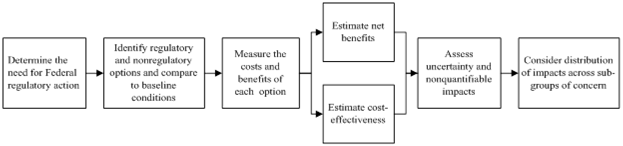
As illustrated in the Figure, Circular A-4 directs that both BCA and CEA be conducted. Additionally, it specifies the following:
■ Monetary valuation of morbidity should ideally be based on estimates of willingness to pay from stated or revealed preference studies, plus any additional economic costs of illness. Preference-based HRQL estimates can be used if WTP studies are not available.
■ Agencies have discretion in the estimates used for the value of a statistical life (VSL)16F[17], however, the Circular cautions about using the value of a statistical life year (VSLY).
■ For effectiveness measures, HALY measures are recommended, along with estimates of discrete physical impacts.
■ Costs and benefits are to be presented undiscounted and discounted at both 3 and 7 percent.
■ Uncertainty should be addressed qualitatively and also in a formal sensitivity analysis; if the regulation’s impact is greater than $1 billion annually, a probabilistic uncertainty analysis is required.
■ Nonquantified benefits and costs of a regulation should be discussed qualitatively in the analysis.
■ Likewise, distributive impacts should be reported and quantified to the extent possible.
Recommended Best Practices of Professional Organizations and Academic Consortia. A variety of papers and policy statements issued by professional organizations and academically based decision analysis researchers and economists have further articulated best practices in economic evaluation and modeling of health and social policy interventions affecting health and well-being. These include:
■ The Principles and Standards for Benefit-Cost Analysis Project at the University of Washington Evans School of Public Affairs, supported by the John D. and Catherine T. MacArthur Foundation (Zerbe et al., 2010)
■ ISPOR-SMDM Joint Modeling Good Research Practices Task Force; papers available:
► Model Parameter Estimation and Uncertainty (Briggs et al., n.d.)
► Model Transparency and Validation (Eddy et al., n.d.)
► Discrete Event Simulation (Stahl et al., n.d.)
► Dynamic Transmission Modeling (Pitman et al., n.d.)
► Conceptual Modeling (Roberts et al., n.d.)
► State-Transition Modeling (Siebert et al., n.d.)
■ Report of the ISPOR Task Force on Good Research Practices—Budget Impact Analysis (Mauskopf et al., 2007)
■ Report of the ISPOR Task Force on Good Research Practices—Randomized Clinical Trials—Cost-Effectiveness Analysis (Ramsey et al., 2005)
■ Report of the ISPOR Task Force on Good Research Practices—Modeling Studies (Weinstein et al., 2003)
Such guidances are indicative of increasing convergence in practice and consensus about rigor and transparency in economic modeling for policy applications.
NICE. The U.K.’s NICE Guideline Development Group (GDG) issues clinical guidelines, for consideration by the National Health Service and local health trusts, based on the best available evidence of both clinical and cost effectiveness (NICE, 2009). The agency directs that guideline recommendations be based on cost effectiveness rather than on budgetary impact. NICE also conducts a separate and parallel cost-impact analysis when the clinical guideline is under consideration, to allow organizations to estimate implementation costs.
The NICE Guidelines Manual states that “An economic analysis will be more useful if it is likely to influence a recommendation, and if the health and financial consequences of the recommendation are large. The value of an economic analysis thus depends on:
■ the overall ‘importance’ of the recommendation (which is a function of the number of patients affected and the potential impact on costs and health outcomes per patient)
■ the current extent of uncertainty over cost effectiveness, and the likelihood that economic analysis will reduce this uncertainty.”
A cost-effectiveness analysis is the preferred form of economic evaluation, using QALYs as the effectiveness metric, if the data are sufficient. Table 3 notes the standards for a reference case CEA that NICE specifies for both technology appraisals and clinical guidelines.
NICE has provisionally proposed using, to provide advice to public health agencies and local health authorities, the following, three-step approach to assessing the returns on investment generated by public health interventions (NICE, 2011): easured in ‘natural’ units. (This and the subsequent CEA would reflect the timing of the costs and benefits – and the sectors in which they occur.
■ A cost–effectiveness analysis with the outcomes expressed in QALYs, to allow comparisons across different program. This preliminary guidance notes that CEAs are not always appropriate for a public health intervention and other methods, such as BCA, may be used.
■ The information from the cost-consequence and cost-effectiveness analyses would be made available to local decision-makers for them to combine with implementation costs and other details, such as eligible population size and the outcome of an assessment of local need, to help them to decide which interventions are priorities.
Recently the U.K. has given greater attention to the cost-effectiveness of public health interventions and surveyed a number of reviews of their economic impact. A group based at the University of York, the Public Health Research Consortium, identified several methodological challenges for evaluating the economic impact of public health interventions: attribution of effects, because of the paucity of controlled trials in public health interventions and the short duration of studies; measuring and valuing outcomes; identifying intersectoral costs and consequences; and incorporating equity considerations (Weatherly et al., 2009). The Consortium’s study of the published reviews and their underlying studies noted that “The existing empirical literature is very disappointing, offering few insights on how to respond to these challenges…there is an urgent need both for pilot studies and more methodological research. (p. 92)”
WHO. In Making Choices in Health: WHO Guide to Cost-Effectiveness Analysis: Methods for generalized cost-effectiveness analysis, Balthussen and colleagues (2003) set out the principles and make the case for an approach to CEA that attempts to overcome disparate methodological practices. Generalized CEA (GCEA) offers an internationally applicable framework for assessing the costs and health benefits of different interventions absent many variable local decision constraints. The authors argue that “sectoral CEA should identify current allocative inefficiencies as well as opportunities presented by new interventions. For this reason, we propose a modification of the standard IMC-[intervention-mix-constrained] CEA, lifting the constraint on the current mix of interventions to evaluate the cost-effectiveness of all options, including currently funded interventions (p.11).”
Two propositions highlight what is distinctive about GCEA. First, evaluate the costs and benefits of a set of related (interactive) interventions against the comparator of the null set of those same interventions. Second, present the results of the analysis in a league table, as the initial step in a policy analysis. Such an array would allow for very broad classification of “very cost-effective,” “very cost-ineffective,” and intermediate interventions, with little significance attached to differential cost-effectiveness ratios within the set of “cost-effective” interventions. Notably, the WHO approach excludes averted costs from the CE ratio.
WHO specifies 14 epidemiological subregions globally for estimating and reporting cost-effectiveness. This approach allows for the application of GCEA by grouping countries (and the CEAs generated for them) within similar health system and epidemiological contexts, and allowing the conditions in the comparator state (the “null set counterfactual”) to be identified. Health impacts are measured in DALYs. The authors emphasize that the set of interrelated interventions that should be removed in the null set counterfactual need not be every health service in local existence; it should, however, include those services whose benefits and costs are overlapping or interactive in some way—or are mutually exclusive.P17F[18]P For example, a GCEA of prevention, screening, and treatment of colorectal cancer included within the set of interrelated interventions a full range of screening modalities with various periodicities; medical treatments for cancer; and a campaign to promote consumption of fruits and vegetables (Ginsberg et al., 2010). Once the GCEA has identified the efficient mix of interventions relative to the null set, the standard IMC-CEA should be used for additional analysis, to inform how to move from the current mix of interventions to the optimal mix.
An Economic Framework for the Prevention of Chronic Diseases. In a working paper commissioned by OECD, Sassi and Hurst (2008) offer an economic framework for considering whether and under what circumstances the prevention of chronic diseases increases social welfare and improves health equity, relative to treatment. They examine the pathways by which chronic diseases emerge, particularly those with behavioral components, and attempt to determine where failures of markets or rationality keep people from achieving the best health outcomes, and where preventive interventions could improve efficiency and equity.
The authors adopt a benefit−cost framework at the broadest level, in view of the twin objectives of improving both social welfare and the equitable distribution of health across a population, and also because of the multiple sectors implicated in the cause and prevention of lifestyle-related chronic diseases. In particular, the framework considers whether and how individual choices in the realm of diet, physical activity, smoking, and drinking involve failures of information (ignorance of consequences), failure to capture externalities of consumption (e.g., in unhealthy foods or education) in their private costs and individual benefits, or failures of rationality (e.g., as with addictive substances). Sassi and Hurst (2008) propose combining BCA with CEA, in order to make the assessment relevant to various decision and budget perspectives, and to separately assess health equity by estimating changes in indicators of health distribution.
The broad scope of this analysis (prevention of any sort of chronic disease with a behavioral component) and the welfare economic framework explicitly consider the achievement of population health goals within the context of other constituents of social welfare, and account for the opportunity costs of prevention efforts. The authors suggest that “The chief contribution to be expected from economic models of health production is…on specific health-related behaviours, particularly in understanding how these contribute to the efficiency of health production and what the interdependencies are between such behaviors and other important health determinants (Sassi and Hurst, 2008, p.20).” They would have a model of health production account for social and environmental influences; life-course factors; general and health-specific education; and uncertainty, time preferences and self-control. Important dimensions within which governments and other actors concerned with developing prevention strategies should classify and evaluate prevention alternatives include the area in which the intervention will be undertaken and the specific health determinants that it is expected to affect, to inform the design, implementation, and funding of the intervention. Another important dimension is the degree to which the intervention interferes with individual choices. Finally, the potential for targeting the intervention should be considered, as the ability to target can potentially affect the efficiency, equity implications, and political feasibility of undertaking the intervention.
In their 2008 discussion, Sassi and Hurst present their work as a guide for more specific policy analyses. This high-level framework helps to identify at a conceptual level the nature of various policy levers in the prevention arena and the kinds of concerns and rationales for choosing among them that a public sector decision maker might need to address.
Section 5. Presentation of Alternative Models in a Summary Framework: Illustrative Topics and Studies
This section presents and discusses economic evaluations grouped according to four health conditions or service type. Because for this project it was not possible to review the literature on preventive services models comprehensively, we limited the search to topics of current policy relevance for which a number of recent economic analyses had been conducted. After reviewing the recommendations of the Advisory Committee on Immunization Practices, the U.S. Preventive Services Task Force, and the Community Preventive Services Task Force—and reviewing our preliminary choices with ASPE—we selected screening mammography to prevent breast cancer; immunization to prevent human papilloma virus (HPV) infection; prevention and management of diabetes; and clinical and community-based interventions to prevent obesity. These topics span primary, secondary and tertiary preventive interventions, represent both clinical and community-based services, and individual analyses represent several forms of analysis: cost of illness, cost-effectiveness, return on investment, and benefit–cost. Thus the range of studies presented here allows for a number of different types of comparisons and contrasts among data sources, model structure, and metrics used.
The review was initially conducted through PubMed using the search terms outlined in Table 4.
41TTable 441T41T.41T Initial Literature Search Criteria
| Health condition | Search terms | Year limitation |
| Breast cancer | mammography AND surveillance AND cost-effectiveness | 2000-present |
| HPV | HPV AND prevent AND (economic OR cost-effectiveness) | 2005-present |
| Diabetes | Diabetes AND prevent AND cost-effectiveness | 2000-present |
| Obesity | obesity AND prevent AND (economic OR cost-effectiveness) | 2000-present |
The abstract list was reviewed by a project co-director and articles of interest were retrieved for a full article review. Additional studies were identified from the reference lists of the pulled studies and reviews of recent journal tables of contents.
Key model characteristics were abstracted from these articles. Model characteristics were chosen prior to abstracting information and were revised according to their suitability to the information presented or if they were deemed useful, post-review. Most retrieved articles were cost-effectiveness analyses; we specifically searched for studies using other model frameworks, such as return-on-investment and benefit–cost analysis. We also identified studies in reviewing national and international guidelines and studies, such as the economic model developed for OECD to estimate the impact of interventions to tackle overweight and obesity at the population level (Sassi et al., 2009).
In order to exhibit models for preventive services most relevant to the geographical region of this project, we have made an effort to include several articles based in the United States (where the literature review may have only yielded one or two US-based articles). However, studies conducted in other countries are informative both in terms of their common features and alternative assumptions. United States-based studies lead each table in descending chronological order, followed by studies conducted in other geographic regions.
The table format was developed iteratively, initially based on the data abstraction form used by the Tufts CEA Registry, and revised to include additional dimensions of economic analyses relevant to comparisons across frameworks. The tables can be found in Section 5.6, following the discussion of each topic in Sections 5.2 through 5.5.
We reviewed four recent economic evaluations of breast cancer screening strategies, one conducted in the U.S. and three in other countries (Spain, Hong Kong, and Japan), presented and referenced in Table 5. Each of these was a CEA; all but one took the perspective of a health care payer or the health care sector overall, and included only direct medical care costs. All four measured either life years extended or QALYs gained, or both. The focus of each of the studies was to ascertain the cost-effectiveness, at least in comparison to no screening, of different periodicities and starting and stopping ages for screening mammography. In the case of the Japanese study, annual clinical breast exam was modeled as an alternative and concurrent intervention.
These studies, published between 2006 and 2011, reveal considerable consistency in model structure (dynamic, Markov chains) and stipulated parameters, such as discount rate, while specific health states and transition paths differed across the studies, both by choice and due to data limitations. For example, the U.S. study, which included multiple risk factors such as age, breast density, previous family history, and prior biopsy in evaluating the cost effectiveness of alternative age thresholds and intervals for screening, excluded women with the BRCA1 or BRCA2 gene from the model.
The relatively recent introduction of both a quadrivalent (types 6, 11, 16 and 18) and a bivalent (types 16 and 18) vaccine for human papilloma virus (HPV) infection, the preponderant cause of cervical cancer, has led to a multitude of possible alternative scenarios of combined immunization and screening interventions. The economic evaluations of HPV and cervical cancer prevention strategies that have been conducted over the past decade have become increasingly complex. Yet little is known about the protection offered by the vaccines over the longer term, which introduces considerable uncertainty into the models for optimizing clinical and cost-effectiveness of mixed prevention strategies.
Table 6 presents abstracted information from 10 CEAs published between 2003 and 2011. Six of the analyses were conducted in the U.S. and one each in France, the Netherlands, Brazil, and Great Britain. This set of studies helps to illustrate a variety of context-specific factors, policy alternatives, and modeling choices in the prevention of cervical cancer.
The non-U.S. studies, for example, illustrate the significance of cervical cancer screening coverage and periodicity in determining the cost-effectiveness of vaccinating pre-adolescent girls against HPV types 16 and 18. Among the group of U.S. studies, in contrast, the comparator, screening cytology, provides a consistent backdrop. The British study by Jit and colleagues (2011) compares the cost-effectiveness of the bivalent and quadrivalent vaccines, including benefits and costs of protection against non-cancer disease endpoints in addition to cancers. Chesson and colleagues (2011) model alternative immunization strategies for females between age 12 and 26 years, and of boys at age 12, with the quadrivalent vaccine. All of the studies except for the Brazilian population, which measured natural endpoints (cases of disease and life expectancy) reported results that used QALYs. Note that the French and Dutch studies use a lower discount rate for benefits than for costs to partially counteract the occurrence of benefits many years into the future.
In a review of models of cervical cancer prevention in developed countries, Kim and colleagues note that
“countries with well-established screening programs will need to consider the potential avertable burden of disease relative to their status quo, the uncertainty in duration of vaccine protection, the relative performance of new screening strategies that utilize HPV DNA testing, the costs associated with different cervical cancer prevention options, and the likelihood of acceptability and uptake (Kim et al., 2008).”
HPV immunization interventions present particularly complex modeling challenges because of epidemiological dynamics at the population level, the long lag time between the intervention and the impact on disease, and the choice of two vaccines with different protective characteristics. Further, the comparator (or complementary intervention) to the immunization intervention can vary, depending on the screening technology (two forms of cytology and HPV DNA testing, under certain conditions). The review by Kim and colleagues (2008) discusses the kinds of inputs that different types of models—static versus dynamic—require and the nature of the information that they can produce. A dynamic model can, for example, take account of patterns of sexual contact, infectiousness of HPV type, and type-specific prevalence within the population. Key model assumptions include vaccine efficacy and immunization coverage rates. Cost-effectiveness is particularly sensitive to assumptions about the persistence or waning of vaccine efficacy over time; published studies have documented the persistence of protective effect for just under a decade, so this is a major source of uncertainty in modeling results.
Today, with immunization of pre-adolescent girls as the background policy, a full range of alternative cervical cancer screening modalities, start ages for screening and its periodicity can be explored (Goldhaber-Fiebert et al., 2008; Kim et al., 2008).
Economic evaluations of preventive strategies addressing the onset and progression of diabetes and related illness encompass more diversity in analytic approaches, interventions, and disease endpoints and outcomes than seen in the cancer screening and immunization examples discussed so far. Table 7 summarizes nine recently published studies that illustrate this wide ranging field. The studies range from primary prevention (Johansson et al., 2009; Roux et al., 2010; Zhuo et al., 2012), to secondary prevention (screening) (Bertram et al., 2010; Chatterjee et al., 2010), to tertiary prevention (disease management) (Huang et al., 2009; Klein et al., 2011; Mullen and Marr, 2010;), to a combination of primary and secondary prevention (Herman et al., 2005). The interventions studied range from broad community-based physical activity interventions, to intensive diet and activity (lifestyle) management, to pharmaceutical and medical interventions, to bariatric surgery.
The most recent study (Zhuo et al., 2012), conducted with a type 2 diabetes simulation model developed by CDC and RTI International, modeled the impact of a targeted community-based lifestyle intervention program for adults at high risk of developing diabetes over a 25-year period, from the perspective of the health care sector overall. The authors found that the intervention was modestly cost-saving for all age groups over the period, reaching a break-even point by the 14PthP year. The study’s sensitivity analysis revealed that the cost of the intervention in the first two years largely drives the net cost impact of the program. In contrast, a comprehensive state-transition Markov model (the CDC Measurement of the Value of Exercise (MOVE) Model) that encompassed seven community-based physical activity interventions and included five disease outcomes, including type 2 diabetes, estimated a cost-effectiveness ratio of $46,914/QALY for a 1-year individually adapted intensive lifestyle modification for persons at high risk of developing diabetes over a lifetime (Roux et al., 2008). Two studies (Bertram et al., 2010; Herman et al., 2005) reported the cost-effectiveness of drug and lifestyle interventions (compared with no intervention) over a lifetime. The U.S. and Australian studies reported similar results, although the U.S. study (Herman et al., 2005) found the lifestyle intervention more cost-effective relative to metformin than did the Australian study (in which multiple drugs were included).
The study by Huang and colleagues (2009) addresses evidence-based medical management of diabetes from the federal health care budgetary perspective. It applies epidemiological modeling to the projection of future direct, federal diabetes-care costs for adults aged 24-85, with an intervention enrolling adults between 24 and 64, comparing 10- and 25-year budget windows. The study demonstrates the significance of following the population with this chronic condition for the longer time period in order to register health care budgetary savings.
The two studies of bariatric surgery as an intervention to reduce BMI in diabetes patients (Klein et al., 2011; Mullen and Marr, 2010) take the perspective of the health care payer, and are structured as an ROI or BCA. Both studies of this highly targeted, expensive intervention, which were conducted over 9 and 7.5 years, respectively, reported that surgical costs had been recouped through lower medical care costs as compared with non-surgical matched cohorts from the plan within 2.2 or 3.5 years, depending on study and type of surgery.P18F[19]P
Economic assessments of clinical or community-based interventions to affect the development or treatment of obesity can be in many respects similar to those of interventions for the prevention or management of type 2 diabetes. Weight loss or BMI is typically an intermediate outcome in the analysis of diabetes interventions. For example, Roux and colleagues (2008), in the analysis of physical activity interventions discussed above, explicitly focused on particular disease endpoints, with weight loss or BMI as an implicit mechanism, to avoid double-counting impact. Conversely, in the models of the economic impact of obesity-related interventions, specific disease endpoints (type 2 diabetes, cancers, cardiovascular events, and conditions) frequently account for the estimated cost savings for reductions in obesity. Table 8 summarizes six recent analyses. One of these (Finkelstein et al., 2008) estimates lifetime medical cost burden as a function of BMI class. Two are policy-oriented models assessing and comparing multiple clinical and community-based strategies to prevent or reduce obesity for European countries (Sassi et al., 2009) and Australia (Carter et al., 2009). The other three include a RoI model for workplace weight loss interventions (Trogdon et al., 2009); a one-year analysis of a school-based physical activity intervention (Wang et al., 2008); and a British study of weight management within primary care settings (Haynes et al., 2010).
The Trogdon article reports on the development of a workplace obesity intervention model that simulates ROI based on specific businesses’ workforce and intervention characteristics. This model is now available on the CDC website as “LEAN Works: Obesity Cost Calculator.” The model relies on a prevalence-based approach to translate weight loss (in BMI units) into expected changes in medical spending and absenteeism. The CDC online calculator allows for the substitution of default values for many of the employer-specific characteristics if that information is missing.
Wang and colleagues report the first-year experience of an after-school physical activity program in lieu of regular after-school care, randomizing 18 elementary schools within one state into nine intervention and nine control sites. The early results of the intervention suggest that students who attended the physical-activity-enriched after school program at least 2 days per week (40% of the time) achieved a percentage reduction in body fat of 0.76 at an additional cost of $317 per student. The clinical significance of a one-percent reduction in body fat, however, has not been established.
Finkelstein and colleagues (2008) present their model for estimating the lifetime medical cost burden of overweight and obesity as an improvement over previous studies that relied on attributable fraction approaches, which include a limited number of diseases and do not account for confounding and interactions among co-present diseases. Notably, this 2008 study distinguishes overweight and two classes of obesity, and estimates excess remaining lifetime medical expenditures at two ages (20 and 65 years), for four subpopulations (white and black men and white and black women). This structure reveals distinctive patterns of lifetime costs by gender, race and BMI class. Because of the inverse relationship between survival and obesity, the difference in lifetime costs for those in the lower and those in the higher obesity classes is less than reported by the same lead author in an earlier, cross-sectional analysis.
Haynes and colleagues (2010) use the 2006 NICE obesity health economic model to evaluate costs and outcomes associated with weight gain for three conditions: type 2 diabetes, coronary heart disease, and colon cancer. The NICE individual-level model generates a simulated population representative of the UK population, followed over a lifetime, with health status and health resource consumption depending on age, gender, and BMI. The evidence-based intervention of practice nurse or other health care worker guided by ‘weight management advisors’ had demonstrated an average 3kg weight loss at 1 year, for the 45 percent of the original participants reporting back, and this was the base case scenario used in the model, with weight assumed to be regained over the following two years, and then returning to the general expected trajectory. In a number of scenarios the model projected that the one-time intervention was cost-saving, and in others had a cost-effectiveness of between £2000 and £2700 per QALY. Mortality impacts were not included.
Both Sassi and colleagues and Carter and colleagues report on models encompassing a wide range of clinical and community-based interventions that address obesity. The OECD working paper (Sassi et al., 2009) assesses the efficiency and distributional impact of interventions to prevent chronic diseases associated with unhealthy diets and sedentary lifestyles. It employs the Chronic Disease Prevention model (CDP), a stochastic microsimulation model, jointly developed by the OECD and WHO. The model can be used to represent a variety of populations and their distinctive characteristics; this set of analyses represents the region of Europe and the costs represent average conditions across the countries making up the region. The CDP uses a causal web of behavioral risk factors for selected conditions. The notion of a causal web allows for more or less immediate influences on the occurrence of disease; risk factors can also influence other risk factors in the same or a different disease pathway. The dietary, physical activity, and combined interventions fall into the broad categories of community-based counseling; counseling in primary care practices; school-based; environmental modification; and other (e.g., media campaigns). The authors modeled the impact of a number of different groupings of interventions, aimed at different ages and mixing broad-based and targeted strategies. The health impacts and cost impacts of the different collections of interventions are shown separately and graphed as cost-effectiveness ratios over time. Outcomes were measured as DALYs. All interventions had favorable cost-effectiveness ratios and some interventions were cost-saving. This analysis is unique among CEAs reviewed for including information on socioeconomic distributional impact. The authors note that “inequalities in age at death appear to be reduced only to a small extent, whereas the extent to which inequalities between socioeconomic groups may be reduced depends crucially on possible differences in the effectiveness of interventions between the relevant groups [and the model assumes equal effectiveness across groups] (p. 58).”
Assessing Cost-Effectiveness in Obesity (ACE-Obesity) is the title of an overarching initiative of the Victorian Department of Human Services, Australia, begun in 2004, to provide state and national policy makers with the “best available modelled evidence on the effectiveness and cost-effectiveness of selected obesity prevention interventions, particularly amongst children and adolescents (Carter et al., 2009, p.2).” Thirteen interventions, ranging from after-school activity programs to reductions of TV advertising of high-fat and high-sugar foods to gastric banding for morbidly obese adolescents were analyzed within a common evaluation design frame and cost-inclusion protocols (e.g., in all cases productivity gains/losses were excluded; time costs for adults/carers were included). Cost-effectiveness ratios are expressed as the Australian dollar cost/DALY saved, with and without offsetting out-year medical cost reductions attributed to the reduction in BMI due to the intervention. Uncertainty testing of the technical parameters (e.g., economic and epidemiological inputs—which the authors distinguish from sensitivity analysis of key programmatic design features—was conducted with simulation modeling with probability distributions around the input variables based on standard errors or the range of values found in the literature. Finally, the ACE approach, which has also been applied for heart disease, cancer, and mental health, includes a 2PndP stage filter that considers the degree of confidence in the model results and broader issues affecting resource allocation decisions. In this case, the criteria used to review results included equity, strength of evidence, feasibility of implementation, acceptability to stakeholders, sustainability, and potential for side effects.
Table 5. Economic Evaluations of Breast Cancer Screening Strategies
| Abstracted information | Schousboe et al. 2011 Personalizing Mammography by Breast Density and Other Risk Factors for Breast Cancer: Analysis of Health Benefits and Cost-Effectiveness | Carles et al. 2011 Cost-effectiveness of early detection of breast cancer in Catalonia (Spain) | Wong et al. 2010 Cost-effectiveness analysis of mammography screening in Hong Kong Chinese using state-transition Markov modeling | Ohnuki et al. 2006 Cost-effectiveness analysis of screening modalities for breast cancer in Japan with special reference to women aged 40-49 years |
| Framework (BCA, CEA, etc.) | CEA | CEA | CEA | CEA |
| Perspective | National health payer | Payer | Societal | Payer |
| Target population | Americans | Catalan/Spanish | Hong Kong Chinese | Japanese |
| Study population (epidemiological) | US women | Catalan or Spanish | Cancer-free Hong Kong Chinese women aged 40 years or older | Japanese women |
| Study population (economic) | 1,000,000 women | Cohort of 100,000 women | 1,000 women | 4 cohorts of 100,000 women for each of 4 strategies, including no screening |
| Intervention(s) | Mammography annually, biennially or every 3 to 4 years with age intervals of 40 to 49, 50 to 59, 60 to 69, 70 to 79 [initial at age 40 years and with breast density of Breast Imaging Reporting and Data System (BI-RADS) categories 1 to 4] | 20 screening strategies by varying the periodicity of mammography screening exams and age intervals: annual or biennial screening with age intervals that started at 40, 45, 50 years and ended at 69, 70, 74 and 79 years | Mammography biennially (initial at age 40 or 50 years and ending at age 69 or 79 years) | Screening strategies: (1) annual clinical breast exam; (2) annual clinical breast exam plus mammogram; (3) biennial clinical breast exam plus mammogram with age intervals of 30-39, 40-49, 50-59, 60-69, 70-79 |
| Comparator(s) | No Intervention | No Intervention | No Intervention | No Intervention |
| Data sources | US Surveillance, Epidemiology, and End Results (SEER) database, Tice et al. (2008), Taplin et al. (1995), Yabroff et al. (2008), Breast Cancer Surveillance Consortium (BCSC), medical literature | Early Detection Program, hospital databases of the IMAS-Hospital del Mar in Barcelona, National Institute of Statistics (INE), Catalan Institute of Statistics (IDESCAT), Catalan Mortality Registry of the Catalan Government's Department of Health, Girona Cancer Registry | US Surveillance, Epidemiology, and End Results (SEER) database, local sources (government gazette, Hospital Authority), private providers, laboratories and suppliers of consumables | Miyagi Prefectural Cancer Registry; annual report on Vital Statistics of Japan; Grant-in-Aid for Cancer Research survey from the Ministry of Health and Welfare |
| Valuation of health benefits ($, QALYs, LYS, cases averted) | Quality-adjusted life years (QALYs) (EuroQol-5D values for Swedish women), number of women screened over 10 years to prevent 1 death from breast cancer | Years of life (YL), quality-adjusted life years (QALYs), lives extended (LE); QALY weights derived from EuroQol EQ-5D | Life expectancy, quality-adjusted life expectancy | Life-years saved, survival duration |
| Costs | Film mammography, direct costs of DCIS (Ductal Carcinoma In Situ) and invasive breast cancer, false-positive results generating additional procedures | Screening mammogram, administrative, early recall mammogram, invasive tests, non-invasive complementary tests, in-hospital, ambulatory visits, chemotherapy, other hospital labs and radiological tests, radiotherapy, hormone therapy (adjuvant tamoxifen) | Screening mammography, follow-up abnormal screens, treatment of invasive of DCIS (Ductal Carcinoma In Situ) and invasive cancer, terminal care, transportation, time | Screening examinations, diagnostic, initial treatment, terminal care (no further specification) |
| Time horizon | Lifetime | Lifetime | 50 years | Lifetime |
| Discount rate (annual) | Costs and benefits 3% | Costs and benefits 3% | Costs and benefits 3% | Costs and benefits 3% |
| Model design (static/dynamic) | Dynamic (Markov microsimulation, probabilistic sensitivity analysis/Monte Carlo simulation) | Dynamic (Markov, stochastic/probabilistic sensitivity analysis) | Dynamic (Markov, probabilistic sensitivity analysis/Monte Carlo simulation) | Dynamic (No further information specified) |
| Sensitivity analysis (parameters) | One-way: DCIS (Ductal Carcinoma In Situ) incidence, breast cancer incidence, mortality, costs and disutility | One or multi-way not specified. Loss of QALYs due to test results' anxiety considered; increased drug costs; longer follow-up times; changed ratio non-invasive tests due to limited estimation information; screening program participation to 50% (vs. 100%); double costs of invasive tests for screen-detected tumors to account for difficulty of detecting non-palpable lesions | One or multi-way not specified. Clinical, cost parameters (no further specification) | One-way: sensitivity and specificity of screening strategy; costs of screening |
| Value of information | N/S | N/S | N/S | N/S |
| Generalizability/scalability of findings |
|
|
|
|
| Distributional or equity analysis | N/S | N/S | N/S | N/S |
| Results | Biennial mammography cost less than $100 000 per QALY gained for women aged 40 to 79 years with BI-RADS category 3 or 4 breast density or aged 50 to 69 years with category 2 density; women aged 60 to 79 years with category 1 density and either a family history of breast cancer or a previous breast biopsy; and all women aged 40 to 79 years with both a family history of breast cancer and a previous breast biopsy, regardless of breast density. Biennial mammography cost less than $50 000 per QALY gained for women aged 40 to 49 years with category 3 or 4 breast density and either a previous breast biopsy or a family history of breast cancer. Annual mammography was not cost-effective for any group, regardless of age or breast density. | Biennial strategies 50-69, 45-69 or annual 45-69, 40-69 and 40-74 were selected as cost-effective for both effect measures (YL or QALYs). The ICER increases considerably when moving from biennial to annual scenarios. Moving from no screening to biennial 50-69 years represented an ICER of 4,469€ per QALY. | Compared to no screening, a single cohort undergoing biennial mammography would cost US$33,200 to $55,400 per QALY saved depending on the age group. Compared to no screening, a multiple cohort undergoing biennial mammography would cost US$32,800 to $38,700 per QALY saved depending the age group. | In women aged 40–49 years, annual combined modality saved 852.9 lives and the cost/survival duration was 3,394,300 yen/year, whereas for biennial combined modality the corresponding figures were 833.8 and 2,025,100 yen/year, respectively. Annual clinical breast examination did not confer any advantages in terms of effectiveness (815.5 lives saved) or cost-effectiveness (3,669,900 yen/year). While the annual combined modality was the most effective with respect to life years saved among women aged 40–49 years, biennial combined modality was found to provide the highest cost-effectiveness. |
| Limitations | Does not apply to women who carry BRCA1 or BRCA 2 mutation; data limitation on screening frequency; modest interrater reproducibility in qualitative BI-RAD classification; used stage distributions by age but not breast density in the absence of mammography results; mortality rates decreased for early detection or improved treatment; film instead of digital mammography | Data limitations - where not available, borrowed from other sources; did not obtain confidence intervals of model outputs; did not consider indirect costs; did not take into account overdiagnosis effects on costs and benefits; DCIS (Ductal Carcinoma In Situ) cases were not included (would increase cost and decrease quality of life) | Did not have aggregate local stage-specific treatment costs for invasive breast cancer (used individual itemized costs); did not evaluate newer technologies to detect breast lesions (MRI, ultrasound, full-field digital mammography or computer-aided detection techniques | Not an RCT; data limitations for sensitivity and specificity of screening |
Table 6. Economic Evaluations of HPV Infection Interventions
Table 7. Economic Evaluations of Diabetes Prevention and Management
Table 8. Economic Evaluations of Interventions to Prevent Obesity
| Abstracted information | Trogden et al. 2009 A return-on-investment simulation model of workplace obesity interventions | Wang et al. 2008 Cost-effectiveness of a school-based obesity prevention program | Finkelstein et al. 2008 The lifetime medical cost burden of overweight and obesity: implications for obesity prevention | Haynes et al. 2010 Long-term cost-effectiveness of weight management in primary care | Sassi et al. 2009 OECD Health Working Paper No. 48 Improving lifestyles, tackling obesity: the health and economic impact of prevention strategies | Carter et al. 2009 Assessing cost-effectiveness in obesity (ACE-Obesity): an overview of the ACE approach, economic methods and cost results |
| Framework (BCA, CEA, etc.) | ROI | CEA | Burden of disease | CEA | CEA | CEA (Assessing Cost-Effectiveness {ACE} in Obesity approach) |
| Perspective | Work organization | Societal | Societal | Payer | Societal | Societal (Providers, Private sector, Non-health sectors) |
| Target population | Americans | Americans | Americans | British | Any country (can be adapted to simulate a specific country) | Australians |
| Study population (epidemiological) | 1,000 employees representative of the working US population | Eighteen elementary schools in Augusta, GA; a total of 601 subjects | Nationally representative civilian noninstitutionalized population | Broad representative of UK population based on age, gender, BMI, etc. | Europeans (intervention by country) | Children and adolescents (aged 5-19) - target age/condition groups varied according to intervention |
| Study population (economic) | Same as above | Same as above | Perspective of a 20 and 65 year old | 1906 patients | Same as above | Australian population of children and adolescents in year 2001 followed over time |
| Intervention(s) | Worksite strategies (based on CDC Community Guide); Weight Watchers; prescription drug coverage; workplace redesign | "Fitogenic" after-school environment that encouraged moderate-to-vigorous physical activity (MVPA) and health snacks while discouraging sedentary behavior | N/A | Counterweight Program for weight management delivered in Family Practice and other settings by practice nurses and health care workers, with initial guidance and facilitation by 'weight management advisers' | Multiple interventions: mass media campaigns, school-based interventions, worksite interventions, fiscal measures, regulation of food advertising to children, compulsory food labeled, physician/dietician counseling | Model is designed to select among specific interventions. Selection criteria: (1) relevance to current policy decision making; (2) availability of evidence to support meaningful analysis (3) potential impact on addressing the problem (4) ability to specify in clear concrete terms (5) inclusion of a mix of intervention (broad & narrow), and across a range of settings (6) consideration of program logic |
| Comparator(s) | No intervention | No intervention | N/A | No program | No intervention | Current practice (assumed to be 'no intervention’) |
| Data sources | CDC 2005 Behavioral Risk Factor Surveillance System, 2005 Current Population Survey, 2005 National Health Interview Survey, 2001-2003 Medical Expenditure Panel Survey, 2003-2004 | National Center for Education Statistics (NCES) | Medical Expenditure Panel Survey 2001-2004; NHIS 1986-2000; National Death Index 1986-2002 | Counterweight Program evaluation, Office of National Statistics, Health Survey for England, Ara et al. (2005), O'Leary et al. (2004) | WHO, NHANES, HSE, Tan Torres et al. (2003) | Country-specific data where possible, health system costs and disease incidence/prevalence patterns |
| Valuation of health benefits ($, QALYs, LYS, cases averted) | Cost-savings | Reduction in percent body fat (%BF) | N/A | quality-adjusted life years (QALYs) | Disability-adjusted life years (DALYs) | Disability-adjusted life years (DALYs), cost offsets (savings in future health sector expenditure: non-health prevention e.g. safer transport systems, personal activities that maintain/improve health, benefits reflected not in health, time) |
| Costs | Medical, absenteeism | Personnel (coordinator salary and payment of program instructors), instructor training (room, food, supplies, compensation), transportation (school buses, administrators), materials (cost of sports equipment, handbooks, activity books, paper, printing, T-shirt | Lifetime medical expenditures (no further specification) | Diabetes, coronary heart disease, colon cancer, Counterweight program | Intervention at the patient level: medicines, visits, hospital stays, individual health education message. Program level: administration, publicity, training, delivery of supplies | Production losses/gains, time, intervention (teachers, materials, equipment)
Valuation of costs: measured in real terms for reference year, CPI to adjust for inflation (not health inflator, since some are outside of health sector) |
| Time horizon | Multi-year (outcomes is in units of annual cost reduction) | 1 year | Lifetime | Lifetime | 100 years | Lifetime or age 100 years |
| Discount rate (annual) | Costs and benefits 3% | N/S | Costs 3% | Costs and benefits 3.5% | Costs and benefits 3% | Costs and benefits 3% |
| Model design (static/dynamic) | Dynamic (No further specification) | Static (no further specification) | Dynamic (simple linear regression) | Dynamic (no further specification) | Dynamic (microsimulation, stochastic/probabilistic sensitivity analysis) | Dynamic (e.g. disease-specific rates for each 5-year age group), Monte Carlo simulation |
| Sensitivity analysis (parameters) | N/A | One-way: per capita usual after-school care costs | One-way not specified.
Multi-way: mortality by BMI class | One-way: mean weight loss from program, time taken to regain any weight lost from program, underlying background weight gain trend | One or multi-way not specified: effectiveness, coverage, socioeconomic status | One or multi-way not specified: results reflecting explicitly the uncertainty of cost, process, outcome and value estimates (usually economic and epidemiological inputs) |
| Value of information | N/S | N/S | No | No | N/S | No |
| Generalizability/ scalability of findings
|
|
|
|
|
|
|
| Distributional or equity analysis | N/S | N/S | N/S | N/S | Sensitivity analysis of socioeconomic status shows less well-off enjoy larger life-year gains. Gini coefficient: all interventions have a favorable but small effect on health equity | Considered in assessment of degree of confidence in CE ratios or broader resource allocation issues |
| Results | Across all over-weight and obese employees, 5% weight loss would result in a reduction in total annual costs (medical plus absenteeism) of $90 per person | Intervention costs were $558/student or $956/student who attended ≥40% of the sessions. Costs net of usual after-school care costs per participating student were $317/student. Students attending ≥40% of the intervention reduced body fat by 0.76% (95% CI: -1.42 to -0.09%) | underweight (BMI: 18.5), low/normal(BMI: 18.5–19.9), normal (BMI: 20–24.9, omitted in specification for reference), overweight (BMI: 25–29.9), obese I (BMI: 30–34.9), obese II/III combined (BMI: >35)
With the exception of white women, the lifetime costs of overweight are around zero. For 20-year-old overweight white women, these costs are estimated at $8,120, with only 11% occurring beyond age 65. From the perspective of a 65 year old, the costs of overweight are $4,560.For 20-year-old obese I adults, lifetime costs range from$5,340 for black women to $21,550 for white women.
For 20 year olds in the obese II/III class, black men have the lowest lifetime cost estimates, $14,580, and white women again have the highest lifetime cost estimates, $29,460. For men, the costs of obese II/III are similar to those of obese I. From the perspective of an obese 20 year old, the percentage of costs occurring after age 65 ranges from 3% for obese II/III black women to28% for obese I black men.
From the perspective of a 65 year old, lifetime costs of obese I range from $4,660 (black women) to $19,270 (black men). For obese II/III, these estimates range from $7,590 (black women) to $25,300 (white women). From this perspective, lifetime costs are higher for the obese II/III class than for those who are obese I. | Even assuming dropouts⁄ non-attenders at 12 months (55%) lost no weight and gained at the background rate, Counterweight was ‘dominant’ (cost-saving) under ‘base-case scenario’, where 12-month achieved weight loss was entirely regained over the next 2 years, returning to the expected background weight gain of 1 kg ⁄ year.
The ICER was £2017/QALY where background weight gain was limited to 0.5 kg ⁄ year, and £2,651 at 0.3 kg ⁄ year.
Under a ‘best-case scenario', where weights of 12-month-attenders were assumed thereafter to rise at the background rate, 4 kg below non-intervention trajectory (very close to the observed weight change), Counterweight remained ‘dominant’ with background weight gains1 kg, 0.5 kg or 0.3 kg ⁄ year. | Most interventions have cost-effectiveness ratios between 0 and $50,000 with two interventions, namely fiscal measures and food advertising self-regulation, generating savings. | The intervention costs varied considerably, both in absolute terms (from cost saving [6 interventions] to in excess of AUD50m per annum) and when expressed as a 'cost per child' estimate (from |
| Limitations | Avoid future obesity-attributable costs; does not account for worker's compensation, disability and insurance costs. and reduced productivity; assumes a stable cohort of employees (higher raters of employee turnovers are likely to realize smaller gains from interventions; in reality, not all firms bear the total costs | Public health significance of %BF is unknown, because studies have tried to define obesity in children by %BF rather than BMI percentiles; intermediary outcome measured, instead of final outcome in terms of health status indicator | Data limitations for estimation and exclusion of other obesity effects, such as use of nursing home care, absenteeism, presenteeism, disability, worker's compensation, and decreased quality of life | Data limitations on background trend in weight gain - although sensitivity analysis shows still cost-effective despite more conservative estimates | Combinations of input data from heterogeneous sources; simplification of relationships among risk factors in mathematical model; assumption of uniform effectiveness across all subpopulation groups (affects distributional analysis results) | Assessment of issues that either influence the degree of confidence that can be placed in the CE ratios, or broader issues that need to be taken into account in decision-making about resource allocation: equity, strength of evidence, feasibility of implementation, acceptability to stakeholders, sustainability, and potential for side effects
Cost offset may be overestimated, since they are based on the mean reduction in BMI; variability in salary structure, health systems, unit costs, implementation method, population size and structure between countries |
This literature review and environmental scan has considered economic models available for the estimation of the benefits of preventive interventions—understanding “models” in terms of very broad types of analytic frameworks employed in the economic evaluation of health-related interventions. It has also considered the needs and constraints of public-sector analysts in applying the results of economic models. Here we present issues and questions in the economic modeling of prevention benefits considered by the expert panel convened at NORC offices in Bethesda, MD, on April 17, 2012. This outline anticipates ongoing work to articulate options and alternatives for HHS both in model construction and for future research.
Much of the work to date in developing models for the economic evaluation of preventive interventions has directly followed the standards for CEA set out in the 1996 report of the Panel on Cost-Effectiveness in Health and Medicine (Gold et al.), which dictates a reference case analysis from the societal perspective. However, in order to address the concerns and questions of federal policy makers—and the budget analysts and actuarial staff that support them—both the data and modeling infrastructures for programmatic and health-sector impacts need focused attention and development for policy applications. Although federal regulatory impact analysis is predominantly BCA, and BCA is used by the legislative review agency in Washington State (Washington State Institute of Public Policy (WSIPP)) to evaluate social policies, CEA remains the leading analytic framework for health care services and public health interventions. Thus our preliminary observations and suggestions for further work in modeling the benefits of prevention primarily refer to practices in CEA.
The following outlines a preliminary set of topics based on the models reviewed and discussions held to date for subsequent development. The expert panel addressed the following overarching questions:
■ Are there ways to make the different perspectives employed in various contexts (regulatory impact assessment, CBO projections, and HHS budgetary analysis) more transparent so that people understand why they can yield different results?
■ What strategies can we develop to improve the transparency of models and their findings?
■ How can best-practice modeling techniques be used by public sector estimators to provide more rigorous projections of both the clinical and spending impact of prevention efforts?
■ Can these models provide the kind of outputs necessary for federal level cost estimates in both the legislative and executive branches?
One of the outcomes of the expert panel meeting was a general acknowledgment of the need for simple tools, criteria, questions, and metrics for the audiences of models to employ in evaluating the models. Despite the various perspectives and traditions followed by different modelers, a common set of standards by which to communicate assumptions and methods would improve transparency and understanding.
The following are more specific issues that the expert panel considered:
Data for modeling prevention benefits. Most trials or evaluations are of limited time scope, which do not capture the participants’ health status and utilization prior to the intervention or after the intervention is over. What can be done to provide a more comprehensive time perspective? Should clinical trials include several years of follow-up data collection? Might clinical trials be designed such that the health care claims experience of participants would be collected and analyzed for a specific period of time (e.g., two years) prior to the intervention and after the trial ends?
Both traditional clinical trials and pilot or demonstration community-based interventions evidence selection effects. Often the study population is chosen for their clinical profile (e.g., absence of comorbidities) or their willingness to participate. This introduces at least some level of selection bias and can complicate the ability of modelers to project the trial or intervention population to broader populations such as all Medicare beneficiaries or the U.S. population overall. A related problem is the under- representation of key policy subpopulations, such as underserved or economically disadvantaged communities, seniors, or children. How can study populations be selected to be representative of the broader population the policy may cover? Can more representative trial/intervention populations be developed?
Academic modelers rely on peer-reviewed sources for price data, whereas federal modelers rely on publicly documented sources such as Medicare payment rates. How are prices estimated where there is neither a peer-reviewed source nor a public rate schedule (e.g., community-based anti-obesity programs)? What inflation rates should be used? When is the consumer price index (CPI) appropriate, the medical care component of the CPI, versus the gross domestic product (GDP) deflator?
How should economic models of preventive interventions address the effects on labor force participation, such as absenteeism, presenteeism, lifetime earnings impacts, retirement decisions, and participation in public income support and social services programs?
Modeling prevention benefits. What are the appropriate time horizons and budget windows for economic models of preventive interventions? What discount rates should apply? Should health benefits far in the future be discounted at the same rate as monetary costs? How should health benefits, including health-related quality of life (HRQL) be measured and expressed? Should preference-weighted HRQL metrics become part of the calculations in policy models?
Can traditional academic models produce and report outcomes that are useful in policy contexts (e.g., in terms of time horizons, discounting practices, measurement and valuation of health states)? Have any new areas of consensus (or disagreements) in the conduct of cost-effectiveness analysis emerged since the 1996 U.S. Panel on Cost-Effectiveness in Health and Medicine report? Has the methodology become more sophisticated to address current limitations? How have or might variation in health state valuations by age or current health condition be addressed? Is any consensus on the treatment of time costs developing?
NORC at the University of Chicago would like to thank the following members of the expert panel who reviewed and offered advice on an earlier draft of this paper:
■ John Bertko, F.S.A., M.A.A.A, Center for Consumer Information and Insurance Oversight (CCIIO),Previous Chief Actuary, Humana
■ Linda Bilheimer, Ph.D, Congressional Budget Office (CBO)
■ Ron Goetzel, Ph.D, Emory University, Thomson Reuters
■ Scott Grosse, Ph.D, Centers for Disease Control and Prevention (CDC)
■ Sandra Hoffman, Ph.D, Resources for the Future Economic Research Service, Department of Agriculture
■ David Holtgrave, Ph.D, Johns Hopkins Bloomberg School of Public Health
■ Lynn Karoly, Ph.D., M.A., RAND
■ William Lawrence, M.D., M.S., Agency for Healthcare Research and Quality (AHRQ)
■ Michael Maciosek, Ph.D, HealthPartners Research Foundation
■ Willard Manning, Ph.D, University of Chicago
■ Peter Neumann, Sc.D, Tufts Medical Center
■ Louise Russell, Ph.D, Rutgers University
■ Jane Kim, Ph.D., M.Sc., Harvard School of Public Health
■ Stephanie Lee, M.A., Washington State Institute for Public Policy (WSIPP)
■ Colin Baker, Ph.D, National Institutes of Health (NIH)
We would also like to thank William Scanlon, Ph.D., GAO (retired); Judith Wagner, Ph.D., CBO (retired); and John Shatto, FSA, Office of the Actuary, CMS, who shared with us their insights about federal modeling practices in the early stages of our work.
Finally, we would like to thank Kevin Haninger, Ph.D., and Amy Nevel, M.P.H., Office of the Assistant Secretary for Planning and Evaluation (ASPE), for their guidance and encouragement in developing this report.
Aljunid, S., Zafar, A., and Saperi, S., et al. (2010). Burden of disease associated with cervical cancer in Malaysia and potential costs and consequences of HPV vaccination. Asian Pacific Journal of Cancer Prevention, 11(6), 1551-1559.
Annemans, L., Rémy, V., and Oyee, J., et al. (2009). Cost-effectiveness evaluation of a quadrivalent human papillomavirus vaccine in Belgium. Pharmacoeconomics, 27(3), 231-245.
Baltussen, R., Adam, T., and Tan-Torres Edejer, T. (2003). Methods for generalized cost-effectiveness analysis. In Making choices in health: WHO guide to cost-effectiveness analysis (pp. 2-122). Geneva: World Health Organization.
Bauch C.T., Anonychuk, A.M., and Pham, B.Z., et al. (2007). Cost-utility of universal hepatitis A vaccination in Canada. Vaccine, 25(51), 8536-48.
Bergeron, C., Largeron, N., and McAllister, R., et al. (2008). Cost-effectiveness analysis of the introduction of a quadrivalent human papillomavirus vaccine in France. International Journal of Technology Assessment in Health Care, 24(1), 10-19.
Bertram, M.Y., Lim, S.S., and Barendregt, J.J., et al. (2010). Assessing the cost-effectiveness of drug and lifestyle intervention following opportunistic screening for pre-diabetes in primary care. Diabetologia, 53(5), 875-878.
Birmingham, C.L., Muller, J.L., and Palepu, A., et al. (1999). The cost of obesity in Canada. Canadian Medical Association Journal, 160(4), 483-488.
Braithwaite, R.S., Meltzer, D.O., and King, J.T., et al. (2008). What does the value of modern medicine say about the $50,000 per quality-adjusted life-year decision rule? Medical Care, 46(4), 349-356.
Brazier, J., Deverill, M., and Green, C., et al. (1999). A review of the use of health status measures in economic evaluation. Health Technology Assessment 3(9):1-164.
Briggs, A.H. (2000). Handling uncertainty in cost-effectiveness models. Pharmacoeconomics, 17(5), 479-500.
Briggs, A., Claxton, K., and Schulpher, M. (2006a). Decision making, uncertainty and the value of information. In Decision modelling for health economic evaluation (pp. 165-200). New York: Oxford University Press, 2006.
Briggs, A. H., Claxton, K., and Schulpher, M. (2006b). Making decision models probabilistic. In Decision modelling for health economic evaluation (pp. 77-120). New York: Oxford University Press.
Briggs, A., Fenwick, E., and Karnon, J., et al. (n.d.). DRAFT-- Model parameter estimation and uncertainty: A report of the ISPOR-SMDM modeling good research practices task force working group --Part 3. Retrieved from International Society for Pharmacoeconomics and Outcomes Research website: Uhttp://www.ispor.org/workpaper/modeling_methods/DRAFT-Modeling-Task-Force_Model-Parameter-Estimation-and-Uncertainty-Report.pdfU
Brisson, M., Van de Velde, N., and Boily, M. (2009). Economic evaluation of human papillomavirus vaccination in developed countries. Public Health Genomics, 12(5-6), 343-351.
Brown, H.S. 3rd, Pérez, A., and Li, Y.P., et al. (2007). The cost-effectiveness of a school-based overweight program. International Journal of Behavioral Nutrition and Physical Activity, 4, 47.
Carande-Kulis, V.G., Maciosek, M.V., and Briss, P.A., et al. (2000). Methods for systematic reviews of economic evaluations for the Guide to Community Preventive Services. American Journal of Preventive Medicine, 18(1S), 75-91.
Carles, M., Vilaprinyo, E., and Cots, F., et al. (2011). Cost-effectiveness of early detection of breast cancer in Catalonia (Spain). BMC Cancer, 11(192). Retrieved from Uhttp://www.biomedcentral.com/content/pdf/1471-2407-11-192.pdfU
Carter, R., Moodie, M., and Markwick, A., et al. (2009). Assessing Cost-Effectiveness in Obesity (ACE-Obesity): an overview of the ACE approach, economic methods and cost results. BMC Public Health, 9(419). Retrieved from Uhttp://www.biomedcentral.com/content/pdf/1471-2458-9-419.pdf
Cecchini, M., Sassi, F., and Lauer, J.A., et al. (2010). Tackling of unhealthy diets, physical inactivity, and obesity: Health effects and cost-effectiveness. Lancet, 376(9754), 1775-1784.
Centers for Disease Control and Prevention (CDC). (2011a). HIV cost-effectiveness. Retrieved from Uhttp://www.cdc.gov/hiv/topics/preventionprograms/ce/index.htmU
Center for Disease Control and Prevention (CDC). (2011b). Obesity Cost Calculator. In CDC's LEAN Works! - A Workplace Obesity Prevention Program. Retrieved from 30TUhttp://www.cdc.gov/leanworks/costcalculator/index.htmlwww.cdc.gov/leanworks/costcalculator/index.htmlU30T
Chapman, R. H., Berger, M., and Weinstein, M. C., et al. (2004). When does quality-adjusting life-years matter in cost-effectiveness analysis?. Health Economics, 13(5), 429-436.
Chatterjee, R., Narayan, K.M. V., Lipscomb, J., et al. (2010). Screening adults for pre-diabetes and diabetes may be cost-saving. Diabetes Care, 33(7), 1484-1490.
Chesson, H. W., Ekwueme, D. U., and Saraiy, M., et al. (2008). Cost-effectiveness of human papillomavirus vaccination in the United States. Emerging Infectious Diseases, 14(2), 244-251.
Chesson, H.W., Ekwueme, D. U., and Saraiya, M., et al. (2011). The cost-effectiveness of male HPV vaccination in the United States. Vaccine, 29(46), 8443-8450.
Chiang, C. L. (1965). An index of health: mathematical models. Washington, D.C.: U.S. Dept. of Health, Education, and Welfare, Public Health Service.
Chisholm, D., and Evans, D. (2007). Economic evaluation in health: Saving money or improving care? Journal of Medical Economics, 10(3), 325-337.
Cooper, B.S., and Rice, D.P. (1976). The economic cost of illness revisited. Social Security Bulletin, 39(2), 21-36.
Coupé, V. M., van Ginkel, J., and de Melker, H. E., et al. (2009). HPV16/18 vaccination to prevent cervical cancer in The Netherlands: model-based cost-effectiveness. International Journal of Cancer, 124(4), 970-978.
de Hollander, A. E., Melse, and J. M., Lebret, E., et al. (1999). An aggregate public health indicator to represent the impact of multiple environmental exposures. Epidemiology, 10(5), 606-617.
Department of Transportation (DOT). (2009). Revised departmental guidance: Treatment of the value of preventing fatalities and injuries in preparing economic analyses. Washington, D.C.
DeVol, R., Bedroussian, A., et al. (2007). An unhealthy America: The economic burden of chronic disease -- Charting a new course to save lives and increase productivity and economic growth. Santa Monica, CA: Milken Institute.
Doubilet, P., Begg, C.B., and Weinstein, M.C., et al. (1985). Probabilistic sensitivity analysis using Monte Carlo simulation. A practical approach. Medical Decision Making, 5(2), 157-177.
Dolan, P., and Edlin, R. (2002). Is it really possible to build a bridge between cost–benefit analysis and cost-effectiveness analysis? Journal of Health Economics, 21(5), 827-843.
Eddy, D. M., Hollingworth, W., and Caro, J. J., et al. (n.d.) DRAFT -- Model transparency and validation: A report of the ISPOR-SMDM modeling good research practices task force working group -- Part 4. Retrieved from International Society for Pharmacoeconomics and Outcomes Research website: Uhttp://www.ispor.org/workpaper/modeling_methods/DRAFT-Modeling-Task-Force_Validation-and-Transparency-Report.pdfU
Eddy, D.M., and Schlessinger, L. (2003a). Archimedes: a trial-validated model of diabetes. Diabetes Care, 26(11), 3093-3101.
Eddy, D.M., and Schlessinger, L. (2003b). Validation of the Archimedes diabetes model. Diabetes Care, 26(11), 3102-3110.
Eddy, D.M., Schlessinger, L., and Kahn, R. (2005). Clinical outcomes and cost-effectiveness of strategies for managing people at high risk for diabetes. Annals of Internal Medicine, 143(4), 251-264.
Elbasha, E. H., Dasbac, E. J., and Insing, R. P. (2007). Model for assessing human papillomavirus vaccination strategies. Emerging Infectious Diseases, 13(1), 28-41
Engelgau, M.M. (2005). Trying to predict the future for people with diabetes: A tough but important task. Annals of Internal Medicine, 143(4), 301-302.
Eubank, S., Guclu, H., and Kumar, V.S., et al. (2004). Modeling disease outbreaks in realistic urban social networks. Nature, 429(6988), 180-4.
Executive Order. No. 12291, 3 C.F.R. 127 (1981).
Fanshel, S., and Bush, J. (1970). A health status index and its application to health services outcomes. Operations Research, 18(6), 1021-1066.
Feinstein, A.H., and Cannon, H.M. (2001). Fidelity, verifiability, and validity of simulation: Constructs for evaluation. Developments in Business Simulation and Experimental Learning, 28, 57-67.
Finkelstein, E.A., Fiebelkorn, I.C., and Wang, G. (2005). The costs of obesity among full-time employees. American Journal of Health Promotion, 20(1), 45-51.
Finkelstein, E.A., Fiebelkom, I.C., and Wang, G. (2003). National medical spending attributable to overcome weight and obesity: how much, and who's paying? Health Affairs (Web Exclusive), W3-219-226.
Finkelstein, E. A., Trogdon, J. G., and Brown, D. S., et al. (2008). The lifetime medical cost burden of overweight and obesity: implications for obesity prevention. Obesity, 16(8), 1843-1848.
Fox-Rushby, J. A., and Hanson, K. (2001). Calculating and presenting disability adjusted life years (DALYs) in cost-effectiveness analysis. Health Policy and Planning, 16(3), 326-331.
Ginsberg, G.M., Lim, S.S., and Lauer, J.A., et al. (2010). Prevention, screening and treatment of colorectal cancer: A global and regional generalized cost effectiveness analysis. Cost Effectiveness and Resource Allocation 8(2).
Gold, M. R., Siegel, J. E., and Russell, L. B., et al. (1996). Cost-effectiveness in health and medicine. New York: Oxford University Press.
Gold, M. R., Stevenson, D., and Fryback, D. G. (2002). HALYS and QALYS and DALYS, Oh My: similarities and differences in summary measures of population health. Annual Review of Public Health, 23, 115-134.
Goldie, S.J., Diaz, M., and Kim, S.Y., et al. (2008). Mathematical models of cervical cancer prevention in the Asia Pacific region. Vaccine, 26, M17-29.
Goldie, S. J., Kim, J. J., and Kobus, K., et al. (2007). Cost-effectiveness of HPV 16, 18 vaccination in Brazil. Vaccine, 25(36), 6257-6270.
Goldie, S. J., Kohli, M., and Grima, D., et al. (2004). Projected clinical benefits and cost-effectiveness of a human papillomavirus 16/18 vaccine. Journal of National Cancer Institute, 96(7), 604-615.
Green, C. (2001). On the societal value of health care: what do we know about the person trade-off technique?. Health Economics, 10(3), 233-243.
Grosse, S.D., Waitzman, N.J., Romano, P.S. et al. (2005). Reevaluating the benefits of folic acid supplementation in the United States: Economic analysis, regulation, and public health. American Journal of Public Health, 95(11), 1917-1922.
Haddix, A. C., Teutsch, S. M., and Corso, P. S. (2003). Prevention effectiveness: A guide to decision analysis and economic evaluation. (2nd ed.). New York: Oxford University Press.
Hammitt, J. K. (2002). QALYs versus WTP. Risk Analysis, 22(5), 985-1001.
Haninger, K., and Hammitt, J. K. (2011). Diminishing willingness to pay per quality-adjusted life year: Valuing acute foodborne Illness. Risk Analysis , 31(9), 1363-1380.
Haynes, S. M., Trueman, P., and Lyons, G. F., et al. (2010). Long-term cost-effectiveness of weight management in primary care. International Journal of Clinical Practice, 64(6), 775-783.
Herman, W.H., Hoerger, T.J., and Brandle, M., et al. (2005). The cost-effectiveness of lifestyle modification or Metformin in preventing type 2 diabetes in adults with impaired glucose tolerance. Annals of Internal Medicine, 142(5), 323–332.
Hirth, R. A., Chernew, M.E., and Miller, E., et al. (2000). Willingness to pay for a quality-adjusted life year: In search of a standard. Medical Decision Making, 20, 332-342.
Huang, E.S., Basu, A., and O'Grady, M.J., et al. (2009). Using clinical information to project federal health care spending. Health Affairs, 28(5), w978-w990.
Irvine, L., Barton, G. R., and Gasper, A. V., et al. (2011). Cost-effectiveness of a lifestyle intervention in preventing Type 2 diabetes. International Journal of Technology Assessment in Health Care, 27(4), 275-282.
Jit, M., Chapman, R., and Hughes, O., et al. (2011). Comparing bivalent and quadrivalent human papillomavirus vaccines: economic evaluation based on transmission model. BMJ, 343, d5775.
Johansson, P., Ostenson, C. G., and Hilding, A. M., et al. (2009). A cost-effectiveness analysis of a community-based diabetes prevention program in Sweden. International Journal of Technology Assessment in Health Care, 25(3), 350-358.
John, J. (2010). Economic perspectives on pediatric obesity: impact on health care expenditures and cost-effectiveness of preventive interventions. Nestle Nutrition Workshop Series Pediatric Program, 66, 111-124.
John, J., Wenig, C.M., and Wolfenstetter, S.B. (2010). Recent economic findings on childhood obesity: cost-of-illness and cost-effectiveness of interventions. Current Opinion in Clinical Nutrition & Metabolic Care, 13(3), 305-313.
Kelly, M. P., Stewart, E., and Morgan, A., et al. (2009). A conceptual framework for public health: NICE’s emerging approach. Public Health, 123(1), e14-20.
Kim, J.J. (2011). The role of cost-effectiveness in U.S. vaccination policy. New England Journal of Medicine, 365(19), 1760-1761.
Kim, J. J., Brisson, M., and Edmunds, W. J., et al. (2008). Modeling cervical cancer prevention in developed countries. Vaccine, 26(10), k76-k86.
Klein, S., Ghosh, A., and Cremieux, P. Y., et al. (2011). Economic impact of the clinical benefits of bariatric surgery in diabetes patients with BMI ≥35 kg/m². Obesity, 19(3), 581-587.
Kling, J. R. (2011). CBO’s use of evidence in analysis of budget and economic policies. Presentation at Annual Fall Research Conference of the Association for Public Policy Analysis & Management. 30TUhttp://www.cbo.gov/publication/42722U30T
Kochi, A. (2006). [Comparison of treatment between TB, AIDS, and malaria from the public health perspective]. Kekkaku, 81(11), 673-9. PMID: 17154046
Koerkamp, B.G., Hunink, M.G., and Stijnen, T., et al. (2007). Limitations of acceptability curves for presenting uncertainty in cost-effectiveness analysis. Medical Decision Making, 27(2), 101-111.
Krupnick, A. K. (2004). Valuing health outcomes: Policy choices and technical issues. Washington, DC: Resources for the Future.
Kulasingam, S. L., and Myer, E. R. (2003). Potential health and economic impact of adding a human papillomavirus vaccine to screening programs. Journal of the American Medical Association, 290(6), 781-789.
Levi, J., Segal, L.M., and Juliano, C. (2008). Prevention for a healthier America: Investments in disease prevention yield significant savings, stronger communities. Washington, DC: Trust for America's Health.
The Lewin Group. (2009). A path to a high-performance U.S. health system: Technical documentation (Rep. No. 47039). Washington, D.C.: The Commonwealth Fund.
Li, G., Zhang, P., and Wang, J., et al. (2008). The long-term effect of lifestyle interventions to prevent diabetes in the China Da Qing Diabetes Prevention Study: a 20-year follow-up study. Lancet 371, 1783–89.
Macal, C. M., and North, M. J. (2006). Introduction to agent-based modeling and simulation. MCS LANS Informal Seminar presented at Argonne National Laboratory, Argonne, IL.
Maciosek, M.V., Coffield, A.B., and Edwards, N.M., et al. (2006). Priorities among effective clinical preventive services: Results of a systematic review and analysis. American Journal of Preventive Medicine, 31(1), 52-61.
Maciosek, M.V., Coffield, A.B., and Edwards, N.M., et al. (2009). Prioritizing clinical preventive services: A review and framework with implications for community preventive services. Annual Review of Public Health, 30, 341-355.
Mauskopf, J.A., Sullivan, S.D., and Annemans, L., et al. (2007). Principles of good practice for budget impact analysis: report of the ISPOR Task Force on good research practices--budget impact analysis. Value Health, 10(5), 336-347.
McKay, M.D., Morrison, J.D., and Upton, S.C. (1999). Evaluating prediction uncertainty in simulation models. Computer Physics Communications, 117(1-2), 44-51.
Meltzer, D. O., Hoomans, T., and Chung, J. W. (2011). Minimal modeling approaches to value of information analysis for health research. (Methods Future Research Needs Report No. 6). Retrieved from Agency for Healthcare Research and Quality, U.S. Department of Health and Human Services website: Uhttp://www.effectivehealthcare.ahrq.gov/ehc/products/197/719/MethodsFRN6_06-28-2011.pdf
Menger, C. (1892). On the origins of money. Economic Journal, 2, 239-255.
Miller, W., Robinson, L. A., and Lawrence, R. S. (Eds.). (2006). Valuing health for regulatory cost-effectiveness analysis. Washington, DC: National Academy Press.
Mishan, E.J. (1971). Cost–benefit analysis: An informal introduction. London: Allen and Unwin.
Moodie, M., Haby, M.M., and Swinburn, B., et al. (2011). Assessing cost-effectiveness in obesity: Active transport program for primary school children--TravelSMART Schools Curriculum program. Journal of Physical Activity and Health, 8(4), 503-515.
Mount Hood 4 Modeling Group. (2007). Computer modeling of diabetes and its complications: a report on the Fourth Mount Hood Challenge Meeting. Diabetes Care, 30(6), 1638-1646.
Mrozek, J. R., and Taylor, L. O. (2002). What determines the value of life? A meta-analysis. Journal of Policy Analysis and Management, 21(2), 253-270.
Mullen, D.M., and Marr, T.J. (2010). Longitudinal cost experience for gastric bypass patients. Surgery for Obesity and Related Diseases, 6(3), 243-248
Murray, C. J., and Acharya, A. K. (1997). Understanding DALYs (disability-adjusted life years. Journal of Health Economics, 16(6), 703-730.
Murray, C. J., and Lopez, A. D. (1996).The global burden of disease: a comprehensive assessment of mortality and disability from diseases, injuries, and risk factors in 1990 and projected to 2020. Cambridge, MA: Published by the Harvard School of Public Health on behalf of the World Health Organization and the World Bank.
Environmental Protection Agency (EPA). (2010). Guidelines for preparing economic analyses. National Center for Environmental Economics (NCEE), Office of Policy, U.S. Environmental Protection Agency (EPA).
National Institute for Health and Clinical Excellence (NICE). (2011). Supporting investment in public health: Review of methods for assessing cost effectiveness, cost impact and return on investment, Proof of concept report. London: NICE.
National Institute for Health and Clinical Excellence (NICE). (2009). Chapter 7: Assessing cost effectiveness. In The guidelines manual (pp. 81-91). London: National Institute for Health and Clinical Excellence (NICE).
National Institute for Health and Clinical Excellence (NICE). (2008). Social value judgments: Principles for the development of NICE guidance (Second Edition). London: National Institute for Health and Clinical Excellence (NICE).
Nixon, J., Stoykova, B., and Glanville, J., et al. (2000). The U.K. NHS economic evaluation database. Economic issues in evaluations of health technology. International Journal of Technology Assessment in Health Care, 16(3), 731-742.
Oddsson, K., Johannsson, J., and Asgeirsdottir, T.L., et al. (2009). Cost-effectiveness of human papilloma virus vaccination in Iceland. Acta Obstetricia et Gynecologica Scandinavica, 88(12), 1411-1416.
Office of Management and Budget (OMB). (2003). Circular A-4, Regulatory analysis. Washington, DC: U.S. Office of Management and Budget.
O'Hagan A, Stevenson M, and Madan J. (2007). Monte Carlo probabilistic sensitivity analysis for patient level simulation models: efficient estimation of mean and variance using ANOVA. Health Economics, 6(10), 1009-23.
Ohnuki, K., Kuriyama, S., and Shoji, N., et al. (2006). Cost-effectiveness analysis of screening modalities for breast cancer in Japan with special reference to women aged 40-49 years. Cancer Science, 97(11), 1242-1247.
Okonkwo, Q.L., Draisma, G., and der Kinderen, A., et al. (2008). Breast cancer screening policies in developing countries: A cost-effectiveness analysis for India. Journal of the National Cancer Institute, 100(18), 1290-1300.
Ormand, B.A., Spillman, B.C., and Waidmann, T.A., et al. (2011). Potential national and state Medicare care savings from primary disease prevention. American Journal of Public Health, 101(1), 157-164.
Patient Protection and Affordable Care Act, P.L. No. 111-148, §2702, 124 Stat. 119, 318-319 (2010).
Patrick, D.L., Bush, J.W., and Chen, M.M. (1973). Methods for measuring levels of well-being for a health status index. Health Services Research, 8(3), 228–245.
Phelps, C.E., and Mushlin, A.J.( 1991). On the (near) equivalence of cost-effectiveness and cost-benefit analysis. International Journal of Technology Assessment in Health Care, 7(1), 12-21.
Pitman, R., Brisson, M., and Fisman, D., et al. (n.d.). DRAFT Dynamic transmission modeling: A report of the ISPOR-SMDM modeling good research practices task force working group- Part 5. Retrieved from International Society for Pharmacoeconomics and Outcomes Research website: Uhttp://www.ispor.org/workpaper/modeling_methods/DRAFT-Dynamic-Transmission-Modeling-Report.pdfU
Prevention Institute, and The California Endowment with the Urban Institute. (2007). Reducing health care costs through prevention (Working Document). Prevention Institute and The California Endowment.
Ramachandran, A., Snehalatha, C., and Yamuna, A., et al. (2007). Cost-effectiveness of the interventions in the primary prevention of diabetes among Asian Indians: Within-trial results of the Indian Diabetes Prevention Programme (IDPP). Diabetes Care, 30(10), 2548-2552.
Ramsey, S., Willke, R., and Briggs, A., et al. (2005). Good research practices for cost-effectiveness analysis alongside clinical trials: the ISPOR RCT-CEA Task Force report. Value Health, 8(5), 521-533.
Reed, W.W., Herbers, J. E., and Noel, G.L. (1993). Cholesterol lowering therapy: What patients expect in return. Journal of General Internal Medicine 8, 591-596.
Rein, D.B., Smith, B.D., and Wittenborn, J.S., et al. (2012). The cost-effectiveness of birth-cohort screening for hepatitis C antibody in U.S. primary care settings. Annals of Internal Medicine, 156 (4), 263-270.
Rein, D.B., Wittenborn, J.S., and Zhang, X., et al. (2012). The cost-effectiveness of welcome to Medicare visual acuity screening and a possible alternative welcome to Medicare eye evaluation among persons without diagnosed diabetes mellitus. Archives of Ophthalmology,130 (5), 607-614.
Rein, D.B., Wittenborn, J.S., and Zhang, X., et al. (2011). The cost-effectiveness of three screening alternatives for people with diabetes with no or early diabetic retinopathy. Health Services Research, 46(5), 1534–1561.
Reynolds, C.W. (1987). Flocks, herds and schools: A distributed behavioral model. ACM SIGGRAPH Computer Graphics, 21(4), 24-34.
Rice, D.P. (1966). Estimating the cost of illness. American Journal of Public Health and the Nation's Health, 57(3), 424–440.
Rice, D.P., and Cooper, B.S. (1967). The economic value of human life. American Journal of Public Health 57(11):1954-1966.
Rice, D.P., Hodgson, T.A., and Kopstein, A.N. (1985). The economic costs of illness: a replication and update. Health Care Financing Review, 7(1), 61-80.
Roberts, M., Russell, L., and Palthiel, A.D., et al. (n.d.). DRAFT - Conceptual Modeling: A Report of the ISPOR-SMDM Modeling Good Research Practices Task Force Working Group—Part 2. Retrieved from International Society for Pharmacoeconomics and Outcomes Research website: Uhttp://www.ispor.org/workpaper/modeling_methods/DRAFT_Modeling-Task-Force_Conceptual-Modeling-Report.pdf
Robinson, L.A. (2007). How US government agencies value mortality risk reductions. Review of Environmental Economics and Policy, 1(2), 283-299.
Robinson, L.A., and Hammitt, J.K. (2011). Valuing health and longevity in regulatory analysis: Current issues and challenges. In D. Levi-Faur (Ed.), Handbook on the politics of regulation (411-421). Cheltenham, UK and Northampton, MA: Edward Elgar.
Rodríguez, C.A., and González, L.B. (2009). [The economic implications of interventions to prevent obesity]. Revista Española de Salud Pública, 83(1), 25-41. Review. Spanish.
Roux, L., Pratt, M., and Tengs, T. O., et al. (2008). Cost effectiveness of community-based physical activity interventions. American Journal of Preventive Medicine, 35(6), 578-588.
Saha, S., Hoerger, T.J., and Pignone, M.P., et al. (2001). The art and science of incorporating cost effectiveness into evidence-based recommendations for clinical preventive services. American Journal of Preventive Medicine, 20(3S), 36-43.
Salomon, J.A. (2010). New disability weights for the global burden of disease. Bulletin of the World Health Organization, 88, 879-879.
Sanders, G. D., and Tair, A. V. (2003). Cost effectiveness of a potential vaccine for human papillomavirus.Emerging Infectious Diseases, 9(1), 37-48.
Sassi, F., Cecchini, M., and Lauer, J., et al. (2009). Improving lifestyles, tackling obesity: The health and economic impact of prevention strategies (Working Paper No. 48). Retrieved from Organization for Economic Co-operation and Development (OECD) website: Uhttp://www.oecd-ilibrary.org/docserver/download/fulltext/5ks5pqlc5jnn.pdf?expires=1327938626&id=id&accname=guest&checksum=05710AFBE47DD87040D05E3F36003F15U.
Sassi, F., and Hurst, J. (2008). The prevention of lifestyle-related chronic diseases: An economic framework. (Working Paper No. 32). Retrieved from Organized for Economic Co-operation and Development (OECD) website: Uhttp://www.oecd.org/dataoecd/57/14/40324263.pdfU
Schelling, T. (1968). The life you save may be your own. In: Chase, Jr., S., ed. Problems in Public Expenditure Analysis. Washington, DC: Brookings Institute.
Schlessinger, L., and Eddy, D.M. (2002). Archimedes: a new model for simulating health care systems—the mathematical formulation. Journal of Biomedical Informatics, 35(1), 37-50.
Schousboe, J. T., Kerlikowske, K., and Loh, A., et al. (2011). Personalizing mammography by breast density and other risk factors for breast cancer: analysis of health benefits and cost-effectiveness. Annals of Internal Medicine, 155(1), 10-20.
Siebert, U., Kuntz, K., and Alagoz, O., et al. (n.d.). DRAFT - State-transition modeling: A report of the ISPOR-SMDM modeling good research practices task force working group- Part 3. Retrieved from International Society for Pharmacoeconomics and Outcomes Research website: Uhttp://www.ispor.org/workpaper/modeling_methods/DRAFT_Modeling-Task-Force_State-Transition-Modeling-Report.pdfU.
Sondhi, M. (2005). Effect of time horizon on incremental cost-effectiveness ratios. Cambridge: Massachusetts Institute of Technology.
Stahl, J., Brennan, A., and Mar, J., et al. (n.d.). DRAFT Modeling using discrete event simulation: A Report of the ISPOR-SMDM modeling good research practices task force working group- Part 4. Retrieved from International Society for Pharmacoeconomics and Outcomes Research website: Uhttp://www.ispor.org/workpaper/modeling_methods/DRAFT-Modeling-Task-Force_Discrete-Event-Simulation-Report.pdfU
Stern, M., Williams, K., and Eddy, D., et al. (2008). Validation of prediction of diabetes by the Archimedes model and comparison with other predicting models. Diabetes Care, 31(8), 1670-1671.
Szucs, T.D., Largeron, N., and Dedes, K.J., et al. (2008). Cost-effectiveness analysis of adding a quadrivalent HPV vaccine to the cervical cancer screening programme in Switzerland. Current Medical Research & Opinion, 24(5), 1473-1483.
Tappenden, P., Chilcott, J.B., and Eggington, S., et al. (2004). Methods for expected value of information analysis in complex health economic models: Developments on the health economics of interferon-beta and glatiramer acetate for multiple sclerosis. Health Technology Assessment, 8(27):iii, 1-78.
Taylor, M. (2009). What is Sensitivity Analysis?. What is...? Series. Retrieved from 30TUhttp://www.medicine.ox.ac.uk/bandolier/painres/download/whatis/What_is_sens_analy.pdfU30T
Tengs, T.O. (2004). Cost-effectiveness versus cost-utility analysis of interventions for cancer: Does adjusting for health-related quality of life really matter? Value in Health, 7(1), 70-78.
Trasande, L. (2011). Quantifying the economic consequences of childhood obesity and potential benefits of interventions. Expert Review of Pharmacoeconomics & Outcomes Research, 11(1), 47-50.
Trasande, L., and Chatterjee, S. (2009). The impact of obesity on health service utilization and costs in childhood. Obesity, 17(9), 1749-1754.
Trogdon, J., Finkelstein, E. A., and Reyes, M., et al. (2009). A return-on-investment simulation model of workplace obesity interventions. Journal of Occupational and Environmental Medicine, 51(7), 751-758.
Trust for America's Health (TFAH). (2008). Prevention for a healthier California: Investments in disease prevention yield significant savings, stronger communities. Washington, DC: Trust for America's Health and the California Endowment.
Ubel, P.A. (2003). What is the price of life and why doesn't it increase at the rate of inflation? Archives of Internal Medicine, 163, 1637-1641.
Ubel, P.A., DeKay, M.L., and Baron, J., et al. (1996). Cost-effectiveness analysis in a setting of budget constraints--is it equitable?. New England Journal of Medicine, 334(18), 1174-1177
U.S. Department of Health and Human Services (HHS). (n.d.) The Health Care Law & You. Retrieved from healthcare.gov website: 30TUhttp://www.healthcare.gov/law/index.htmlU30T.
U.S. Department of Health and Human Services (HHS) (2011). Fact sheet: Affordable Care Act rules on expanding access to preventive services for women. Retrieved from healthcare.gov website: Uhttp://www.healthcare.gov/news/factsheets/2011/08/womensprevention08012011a.htmlU
U.S. Department of Health and Human Services (HHS). (2010). Fact sheet: Investing in prevention: The new national prevention, health promotion and public health council. Retrieved from healthreform.gov website: Uhttp://healthreform.gov/newsroom/preventioncouncil.htmlU
U.S. Preventive Services Task Force. (2008). USPSTF Procedure Manual. Retrieved from 30TUhttp://www.uspreventiveservicestaskforce.org/uspstf08/methods/procmanual5.htmU30T.
Usher, C., Tilson, L., and Olsen, J., et al. (2008). Cost-effectiveness of human papillomavirus vaccine in reducing the risk of cervical cancer in Ireland due to HPV types 16 and 18 using a transmission dynamic model. Vaccine, 26(44), 5654-5661.
Wadden, T. A., Neiberg, R. H., and Wing, R. R., et al. (2011). Four-year weight losses in the Look AHEAD study: factors associated with long-term success. Obesity, 19(10), 1987-1998.
Wang, L. Y., Gutin, B., and Barbeau, P., et al. (2008). Cost-effectiveness of a school-based obesity prevention program. Journal of School Health, 78(12), 619-624.
Wang, L.Y., Yang, Q., and Lowry, R., et al. (2003). Economic analysis of a school-based obesity prevention program. Obesity, 11(11), 1313-1324.
Washington State Institute of Public Policy (WSIPP). (2012). Homepage. Retrieved from 30TUhttp://www.wsipp.wa.gov/default.aspU30T.
Weinstein, M.C. (2008). How much are Americans willing to pay for a quality-adjusted life year? Medical Care, 46(4), 343-345.
Weinstein, M.C., O’Brien, B., Hornberger, J., et al. (2003). Principles of good practice for decision analytic modeling in health-care evaluation: Report of the ISPOR task force on good research practices—modeling studies. Value Health, 6(1), 9-17.
Weinstein M.C., Siegel J.E., Gold M.R., et al. (1996). Recommendations of the panel on cost-effectiveness in health and medicine. JAMA, 276(15),1253-1258.
Weinstein, M.C., and Stason, W.B. (1977). Foundations of cost-effectiveness analysis for health and medical practices. New England Journal of Medicine, 296(13), 716-721.
Wikipedia. (n.d.). Comparison of agent-based modeling software. Retrieved from Wikipedia website: Uhttp://en.wikipedia.org/wiki/Comparison_of_agent-based_modeling_softwareU.
Wittenborn, J.S., & Rein, D.B. (2011). Cost-effectiveness of glaucoma interventions in Barbados and Ghana. Optometry & Vision Science, 88(1), 155-163.
Wong, I.O., Kuntz, K.M., and Cowling, B.J., et al. (2010). Cost-effectiveness analysis of mammography screening in Hong Kong Chinese using state-transition Markov modeling. Hong Kong Medical Journal, 16(3), 38-41.
World Health Organization (WHO). (2003). Making Choices in Health: WHO Guide to Cost-Effectiveness Analysis. Geneva, Switzerland: World Health Organization.
World Health Organization (WHO). (2009). WHO guide to identifying the economic consequences of disease and injury. Geneva, Switzerland: World Health Organization, Department of Health Systems Financing Health Systems and Services.
World Health Organization (WHO), Harvard University, Institute for Health Metrics and Evaluation at the University of Washington, John Hopkins University, and University of Queensland. (2009). Global Burden of Diseases (GBD): Study operations manual. Retrieved from Institute for Health Metrics and Evaluation website: Uhttp://www.globalburden.org/GBD_Study_Operations_Manual_Jan_20_2009.pdf
Viscusi, W.K., and Aldy, J.E. (2003). The value of a statistical life: A critical review of market estimates throughout the world. Journal of Risk and Uncertainty, 27(1), 5 – 76. Draft at: Uhttp://yosemite.epa.gov/ee/epa/eermfile.nsf/vwAN/EE-0483-09.pdf/$File/EE-0483-09.pdfU.
Yamamoto, N., Mori, R., and Jacklin, P., et al. (2012). Introducing HPV vaccine and scaling up screening procedures to prevent deaths from cervical cancer in Japan: a cost-effectiveness analysis. BJOG: An International Journal of Obstetrics and Gynaecology, 119(2), 177-186.
Zechmeister, I., Blasio, B.F., and Garnett, G., et al. (2009). Cost-effectiveness analysis of human papillomavirus-vaccination programs to prevent cervical cancer in Austria. Vaccine, 27(37), 5133-5141.
Zerbe, R. O. Jr., Davids, T.B., and Garland, N., et al. (2010). Toward principles & standards in the use of benefit-cost analysis. University of Washington, Benefit-Cost Analysis Center.
Zhuo, X., Zhang, P., and Gregg, E.W., et al. (2012). A nationwide community-based lifestyle program could delay or prevent type 2 diabetes cases and save $5.7 billion in 25 years. Health Affairs, 31(1), 50- 60.
[1] Such bodies include the Office of Management and Budget for regulatory impact assessment; the Community Preventive Services Task Force; and WHO-CHOICE, among others.
[2] Productivity losses may be overestimated because it assumes full employment when in reality unemployed labor is likely to be available.
[3]Cancers, diabetes, heart disease, pulmonary conditions, hypertension, stroke, mental disorders.
[4] Levi et al., 2008, reports state-level projections also.
[5] The application of this concept to the valuation of health impacts was introduced by Schelling (1968) and Mishan (1971).
[6] Some federal agencies, including FDA, use monetized HALY metrics (Miller et al., 2006).
[7] See Robinson and Hammitt (2011) and Robinson (2007), for overviews of federal agencies’ use of VSL.
[8] This section draws on research conducted for and reported in the Institute of Medicine study, Valuing Health for Regulatory Cost-Effectiveness Analysis, 2006, Miller, Robinson and Lawrence, eds.
[9] See additional discussion of the differences between HALY measures and WTP in Hammitt (2002) and Krupnick (2004).
[10] CEAs using HALY metrics are often referred to as cost–utility analyses.
[11] In the second edition of Social Value Judgments: Principles for the development of NICE guidance, NICE says the following: “NICE has never identified an ICER [incremental cost-effectiveness ratio] above which interventions should not be recommended and below which they should….NICE should explain its reasons when it decides that an intervention with an ICER below £20,000 per QALY gained is not cost effective; and when an interventions with an ICER of more than £20,000 to £30,000 per QALY gained is cost effective.”
[12] The PCEHM also encouraged analysts to conduct sensitivity analyses using discount rates ranging from 0 to 10 percent.
[13] A comprehensive review would also include the economic evaluation guidelines of several other national agencies, such as the Canadian Agency for Drugs and Technologies in Health (CADTH), Germany’s Institute for Quality and Efficiency in Health Care (IQWiG), and several Australian agencies, including the Pharmaceutical Benefits Advisory Committee (PBAC).
[14] The USPSTF no longer considers cost effectiveness in making recommendations. This column reflects the guidance for systematic reviews of economic analyses published in 2001 (Saha et al.)
[15] Results are summarized for decision makers through a scoring system that provides values for clinically preventable burden and cost effectiveness for each preventive health service and then assigns a weighted total score to each service.
[16] Figure 7 taken from Miller et al. eds, 2006.
[17] The value of a statistical life refers to the value of small reductions in risk spread throughout a large population; it is not the value of saving the life of an identifiable individual.
[18] WHO’s proposed intervention clusters include categories such as respiratory infections, diarrheal diseases, vaccine-preventable diseases, antenatal/perinatal care and other reproductive health services, cancers, cardiovascular disease including stroke, diabetes, neuro-psychiatric disorders, infectious diseases, and injuries (Annex B, WHO Guide to Generalized Cost-Effectiveness Analysis, 2003).
[19] In Mullen and Marr (2010), the control group was drawn from a time period prior to the surgical intervention, with costs trended forward.