
Final Technical Report for DHHS Contract HHSP23320054301ER
Please do not circulate without permission of the authors or the Office of the Assistant Secretary of the Department of Health and Human Services.
January 21, 2007
Stephen T. Parente, Ph.D.
Roger Feldman, Ph.D.
CARLSON
SCHOOL OF MANAGEMENT
__________________
UNIVERSITY OF MINNESOTA
ABSTRACT
The focus of this study was on the non-price program features that influence the enrollment of non-elderly adults into voluntary state and local programs that subsidize coverage or care. The study consisted of two phases -- Phase 1 was a literature review to assess the current state of knowledge regarding the impact of non-price design features on enrollment. Information gathered from this literature was used to inform Phase 2, which consisted of discussions with 67 program directors and other key informants from 17 subsidized coverage programs across the country. The key findings of the study are as follows:
- There is inadequate knowledge to guide program designers
- Outreach is critical
- A broad spectrum of partnerships is key for creating awareness that leads to enrollment
- Applicants need a high level of insurance counseling and applications assistance
- Program officials need to manage expectations and avoid negative perceptions
- Programs that target adults directly attract enrollment much more easily than programs that involve employers
Material contained in this publication is in the public domain and may be reproduced, fully or partially, without permission of the Federal Government. The courtesy of attribution is requested. The recommended citation follows:
Office of Health Policy, ASPE(2008) Continuation of Research on Consumer Directed Health Plans: HSA Simulation Model Refinement. Washington, DC: U.S. Department of Health and Human Services, Office of the Assistant Secretary for Planning and Evaluation.
Executive Summary
High-deductible health plans (HDHPs) are attracting attention from consumers, employers, and policy-makers. These plans couple a large out-of-pocket deductible with a tax-advantaged health savings account (HSA) that can be used to pay for eligible medical expenses. If an enrollee spends all of the dollars in the HSA in a given year, she then spends her own money until the deductible requirement in the health insurance plan is met. This benefit design can be tailored to cover all or part of the expenditures that exceed the deductible. To facilitate informed decision-making, the enrollee may be provided with information about health care providers, including physician education and experience, prices and quality ratings.
This plan type has been the subject of a public policy discussion as a health insurance mechanism to reduce the number of uninsured by providing financial incentives to consumers to "take-up" consumer driven health plans. Our current results show that these initiatives may hold some promise in reducing the number of uninsured by several million.
In a previous report for the Office of the Assistant Secretary (OASPE) of the Department of Health and Human Services (DHHS), we simulated the effect of the Medicare Modernization Act of 2003 (MMA) on take-up of high-deductible health plans in the individual health insurance market. (Feldman, Parente, Abraham et al, 2005; Parente et al, Final Technical Report for DHHS Contract HHSP233200400573P, 2005) We also simulated the impact of additional subsidies for HDHP enrollment, including one based on our interpretation of the Administration's 2004 proposal that featured low-income tax credits for the purchase of HDHPs. We predicted that proposal would have increased HDHP take-up and reduced the uninsured by 2.9 million people at a tax cost of $8.1 billion per year, or an average tax cost of $2,761 per person.
We contracted with OASPE to extend and refine the simulations that were performed under our prior contract. In particular, we refined the health plan choice model by incorporating the effect of prior health status on health plan choice - a necessary step if one wants to predict enrollment more accurately. Using the results of our choice model, we predicted health care costs for the people who enrolled in each plan. We turned costs into premiums by adding a loading fee and then predicted choices again with the new premiums. We continued to "iterate" the choice model until premiums and choices converged.
In addition to these refinements in the model, we also refined our method for estimating the tax cost of various subsidy proposals to include an offsetting reduction in tax subsidies for people who drop subsidized employer-sponsored health insurance (ESI). Finally, we brought the simulations "up-to-date" by simulating the proposals outlined in the President's 2006 State of the Union (SOTU) speech and explained in detail in the 2006 Treasury Blue Book.1 As we understand that proposal, it has three related parts:
- Tax treatment of HDHP premiums: Individuals covered by an eligible HDHP2 would be allowed an “above-the-line" deduction in determining their adjusted gross income. In order to further level the playing field between individual health insurance and ESI, individuals covered by an eligible HDHP would receive a refundable tax credit equal to the lesser of: (1) 15.3 % of the HDHP premium or (2) 15.3% of their wages subject to employment taxes.
- Tax treatment of HSA contributions: The amount that could be contributed before taxes to the HSA would be increased to the out-of-pocket limit for the individual's HDHP (currently, $5,250 for single coverage and $10,500 for family coverage). This provision would allow covered individuals to pay all out-of-pocket expenses under the HDHP with pre-tax dollars. In addition, individuals making after-tax contributions to the HSA would be allowed an employment tax credit similar to the premium credit described in #1 above.
- Low-income tax credit: A refundable tax credit would be offered to low-income individuals and families to purchase an eligible HDHP. The credit would provide a subsidy of up to 90 % of the health insurance premium, up to a maximum dollar amount, and it would be phased down to zero at higher incomes. Full details of the credit are provided in the 2006 Treasury Blue Book.
The results of our revised simulation of the three policy changes combined, as well as individual impacts, are presented in Exhibit 1. The numbers reflect only the individual market since the group market is offered insurance. Likewise, the uninsured total reflects results from only the individual market. Subsidy costs are tallied for the individual market to give a national presentation of the cost per newly-insured person resulting from the SOTU policies. The least expensive option, per capita, is a tax-deductible HDHP premium. The most expensive is increasing the tax-deductible threshold for the HSA. Interestingly, the per capita cost of the tax credit proposal and entire SOTU are nearly identical.
| HSA Enrollees | Uninsured | New Insured | AnnualSubsidy Cost (millions) | Subsidy Cost per New Insured | |
|---|---|---|---|---|---|
| 2003 Medicare Modernization | 3,272,521 | 27,305,770 | 0 | $0 | $0.00 |
| State of the Union 2006 | 16,194,845 | 17,802,877 | 9,502,893 | $21,829 | $2,297.12 |
| Tax deductible HSA premium | 7,474,963 | 24,420,419 | 2,885,351 | $5,136 | $1,780.09 |
| More deductible HSA contribution | 3,433,760 | 27,214,791 | 90,979 | $393 | $4,316.63 |
| Low income subsidy of HSA premium | 11,929,312 | 20,848,203 | 6,457,568 | $14,792 | $2,290.66 |
It is important to note that these three components are not additive because of the way in which the simulation is calculated. Each component is the result of a separate simulation. Also, our model use 2006 premium estimates. At this time, we do not premium estimates to identify a pre-MMA population (with 2003 premium estimates).
In summary, tax credits for high deductible health insurance premiums would reduce the number of uninsured. That result, combined with the additional proposed policy change of making the HDHP premium tax-deductible, would lead to an even sreater reduction in the uninsured. Increasing the limit of tax-deductible contributions to the HSA has little public policy impact and is the most expensive policy of the three outlined in the SOTU. Combined, the new policy options can have significantly more impact than the previous 2004 proposal with a reduction in the estimated per capita subsidy cost. Of the three proposals, the most impact is produced by the tax credit proposal. The least costly per capita proposal is the tax-deductibility of the HDHP premium. The tax credit and premium deduction policies appear to have largely independent effects. If the HSA contribution proposal is eliminated as an option, the tax credit and premium deduction components could be enacted in stages and not crowd out much of the other's effect. If the goal is to maximize the reduction in the number of uninsured, pursuing the 2006 proposal could reduce the uninsured by nearly 10 million persons, affecting over one third of the individual market.
I. Introduction
Consumer directed health plans (CDHPs) are recent development in the US health insurance market. Their principal economic aim is to make the consumer more engaged in health care purchasing decisions through the provision of an account from which medical services can be purchased. This system is tied to traditional indemnity insurance, usually in the form of a high deductible health plan (HDHP) with a deductible gap of roughly the size of the account - though there are many variations.
A. Prior Study
In a previous report for the Office of the Assistant Secretary (QASPE) of the Department of Health and Human Services (DHHS),3 we simulated the effect of the Medicare Modernization Act of 2003 (MMA) on take-up of HDHP in the individual health insurance market. High deductible health plans feature a large deductible coupled with a Health Savings Account (HSA) owned by the individual that can be used to pay for eligible medical expenses. The MMA made it possible for contributions to the HSA to be made on a tax-preferred basis. That is, contributions less than the size of the deductible are exempt from federal income taxes. If the contribution is made by an employer, it is exempt from Social Security taxes as well. Assuming no additional tax policy incentives are offered for HDHP enrollment, we predicted that there could be approximately 3.2 million HDHP-covered lives among the U.S. population between the ages of 19-64 who are not students, not eligible for coverage under employer-sponsored health insurance, and not enrolled in public health insurance programs.
We also simulated the impact of additional subsidies for HDHP enrollment, including one based on our interpretation of the Administration's 2004 proposal that featured low-income tax credits for the purchase of HDHPs.4 Our model predicted that proposal would have increased HDHP take-up and reduced the uninsured by 2.9 million people at a tax cost of $8.1 billion per year, or an average tax cost of $2,761 per person newly insured.
B. Current Study
In October of 2005, we contracted with OASPE to extend and refine the simulations that were performed under our prior contract. There were three major aspects to this work:
- First, we refined the baseline simulations with a more realistic approach for determining the amount of money that individuals and families contribute to their HSAs. Specifically, we let HSA contributions vary by age and income of the policyholder, while constraining the overall average contribution to be the same as in our previous report. We also refined the health plan choice model by incorporating the effect of prior health status on health plan choice - a necessary step if one wants to predict enrollment more accurately.
- Second, we extended the simulation approach to include an "iterative" model for determining premiums and health plan choices. Using the results of our baseline choice model, we predicted health care costs for the people who enrolled in each plan. We turned costs into premiums by adding a loading fee and then predicted choices again with the new premiums. We continued to "iterate" the model until the predicted premiums did not change from one round to the next. The new outcomes in terms of premiums and enrollment represent a true equilibrium for the simulation model.
- Third, we brought the simulations "up to date" by simulating the proposals outlined in the
President's 2006 State of the Union (SOTU) speech and explained in detail in the 2006 Treasury Blue Book.5 In this step we introduced a more sophisticated method for estimating the tax cost of various subsidy proposals by including an offsetting reduction in tax subsidies for people who drop subsidized employer-sponsored health insurance (ESI) to purchase an individual HDHP policy.
II. Refine Baseline Simulations
To complete our current study, we needed to revise and extend our methods. We also used additional data sources and elements to more fully account for the health status of individuals in our models using claims data from the employers participating in our consumer driven health plan analysis.
A. Methods
There are three major components to our methodological approach: 1) Model Estimation; 2) Choice Set Assignment and Prediction; and 3) Policy Simulation. As illustrated in Figure 1, often more than one database was required to complete the task. Integral to this analysis was the use of consumer directed health plan data from four large employers working with the study investigators.
Figure 1
Figure 1 illustrates the three major components to our methodological approach: 1) Model Estimation; 2) Choice Set Assignment and Prediction; and 3) Policy Simulation. This particular model shows that more than one database was required to complete the task. Several steps were need for this model estimation.
The model estimation had several steps. As a first step, we pooled the data from the four employers offering CDHPs to estimate a conditional logistic plan choice model similar to our earlier work (Parente, Feldman and Christianson, 2004). In the second step we used the estimated choice-model coefficients to predict health plan choices for individuals in the MEPS-HC. In order to complete this step, it was necessary first to assign the number and types of health insurance choices that are available to each respondent in the MEPS-HC. For this purpose we turned to the smaller, but more-detailed MEPS Household Component-Insurance Component linked file, which contained the needed information. The third step was to generate 2006 HSA premiums and benefit designs. The final step was to apply plan choice models coefficients to the MEPS data with premium information as well as 2006 State of union tax treatment adjustments to get final estimates of take up and subsidy costs.
This process was similar to our previous work and described in more detail in the appendix. Two of the most substantial of several changes were inclusion chronic illness into the plan choice model and generation of premiums through an iterative process using prior years claims data to create actuarially fair estimates of premium. Below we describe in more detail specific issues that we addressed in our current analysis.
1. HSA Contributions
To be consistent with our previous work, in the new baseline simulations we assumed that individual HDHP policies had deductibles of $3,500 per year for single coverage and $7,000 for family coverage, and no cost-sharing (i.e. zero coinsurance) once the deductible is met. We also assumed that individuals enrolled in a single-coverage HDHP would contribute $1,000 per year on average toward their HSA, and those with family coverage would contribute $2,000 on average. However, we made a significant change from our previous report where we assumed that everyone with the same coverage type (single or family) would make the same HSA contribution. In the current simulations we relaxed that assumption by allowing HSA contributions to be roughly proportionate to enrollee age and income. Our rationale for this change is that high-income enrollees will find the tax advantages of larger HSA contributions more appealing, and that older enrollees with higher medical care use will want to make larger HSA contributions. Even though we allowed enrollee contributions to differ by age and income, we constrained the average HSA contribution to be $1,000 for single coverage and $2,000 for family coverage. This means that any change in HDHP take-up from our previous simulations would be due to a change in the composition of the contributions, not to a general increase in the contribution level.
The following table shows the matrix of 16 HSA contribution cells we used, where each cell represents a quartile of the age and income distribution of the eligible U.S. population:
| Age | |||||
|---|---|---|---|---|---|
| Income | Quartile | 1st | 2nd | 3rd | 4th |
| 1st | 0 | $100 | $500 | $1,000 | |
| 2nd | 0 | $200 | $800 | $1,500 | |
| 3rd | $50 | $400 | $1,500 | $2,500 | |
| 4th | $100 | $500 | $2,000 | $3,760 | |
Cell values for family-coverage HAS contributions were double those shown above, except in the highest income/oldest age cell, where the family contribution was $8,320. The population- weighted average of the cell values was $1,000 for single coverage and $2,000 for family coverage.
Next, we defined the initial premium variables that were used in the baseline simulations. Each premium had two components: the insurance premium and the tax adjusted HSA contribution as constructed above. Further description of each component of the premium is provided next.
- Premiums for individual HDHP policies were taken from the eHealthinsurance.com web site, which provides a monthly estimated premium cost based on county of location, age, family size, and health history. For single-coverage contracts, we assumed the "baseline" demographic category was a 40-year old, non-smoking male. For family contracts, we assumed the policyholder was a non-smoking, 40-year old married man with a spouse and two children under the age of 10. Premiums for other age groups were age-adjusted using information from a 2002 HIAA/eHealthinsurance.com survey of plans purchased in the individual market. Premiums were updated to 2006 using the medical care component of the Consumer Price Index from the Bureau of Labor Statistics web site.
- Premiums for "traditional" HMO and PPO health plans were taken from the linked 2001
MEPS data file, adjusted for coverage type, plan type, establishment size, and benefits.
Premiums for employer-sponsored HDHP were based on the four employers in our data base. Premium estimates for individual HMO and PPO plans used the adjustment for the smallest establishment size category, based on the assumption that this most closely approximates the loading charge for plan administrative costs in individual health insurance policies. Once we estimated the premiums we inflated them from 2001 to 2006 prices based on medical insurance price inflation during the period.
- We considered the HSA contribution to be similar to a premium because each individual chooses to make that contribution "up front" - just as he or she pays the monthly premium for insurance coverage. However, unlike the monthly premium for insurance coverage, the HSA contribution is made with pre-tax income up to a cap. Therefore, we converted the contribution into pre-tax dollars by multiplying times one minus the personal federal tax rate based on the policyholder's income. We could not adjust for state income tax subsidies because the linked MEPS survey does not identify the respondent’s state of residence.6 We capped the tax subsidy at $2,700 for individual coverage and $5,400 for family coverage, which are the limits specified by current law. The actual contribution was also in effect capped by our range of age and income related premium contributions.7 These caps are binding only for individuals in the highest income/oldest age cell. Consequently, the “premium” variable used in our baseline simulations equals the monthly insurance premium plus the tax-adjusted HSA contribution subject to the cap as described above.
2. Health Plan Choice Model
In the new baseline simulations, we made an important improvement to the health plan choice model by including the effect of health status as a variable that affects plan choice. This is important for two reasons. First, health status may be an important factor in predicting plan choice, so the addition of this variable should improve the fit of the choice model, other things equal. Second, it may be that case that sick (healthy) people prefer certain plans, which would drive the premiums up (down). Specifically, if sick people are attracted to traditional plans, it could lead to a "death spiral" of increasing premiums and falling enrollment for the traditional plans. One of our goals in the new simulations is to determine whether the addition of a HDHP as a choice will tend to de-stabilize the market for health insurance.
To account for health status, we used the claims data for contract holders (employees) in the employers we examined in our prior plan choice analysis. For this analysis, we obtained the claims data for the year prior to their possible enrollment in a high deductible health plan. We used the diagnosis code information from these prior year claims records to calculate a set of 34 Adjusted Diagnosis Groups (ADGs) using a methodology developed by Johns Hopkins University researchers.8 Several of these 34 ADGs identify a diagnosis indicating the presence of a chronic condition. With this information we constructed a dummy variable indicating the presence of chronic illness. This variable construction permitted us to develop a medical care cost regression model to predict future medical expenditure of the MEPS population enrolled in each plan type. A description of the results of these prediction regressions (for each plan choice) is presented in the appendix. Using an aggregate measure of health status represented as a binary variable allowed us to create a variable we could map from the MEPS database in order to predict health plan choice.
The final health plan choice model is presented in the appendix. Besides the inclusion of health status, we also interacted premium and cost sharing variables with more demographic variables. These interactions were introduced to account for possible associations not accounted for by the own-price response to premium and cost sharing variables.
B. Baseline Simulation Results
Table 2 shows the results of the baseline simulation prior to iterations. We predict that approximately 3.2 million people who are not eligible for employer-sponsored health insurance (ESI) will choose an individual HDHP. This estimate was calibrated to be the same as our previous analysis in order to compare the proposed policy changes in 2004 to the 2006 State of the Union proposals.9 An additional 47,509 people will turn down their employers' offers of coverage to purchase an individual HDHP. This is fewer than the 365,150 people who were predicted to "opt out" of ESI in our original simulation of the MMA effects (Parente, et al., 2005). The large swing was attributable to a difference in the tax treatment of the premium in the original analysis that was clarified and corrected in the current study. As a result, we believe our original analysis significantly overstated the likely opt-out of the employer market into individual HSAs.
We predict that only 67,812 people will choose an employer-sponsored HDHP. This is also fewer than the 334,938 individuals who chose this option in the original simulations. Once again, this change was the result of an inaccurate assessment of the tax treatment of the employer sponsored HDHP. We are confident our current model better reflects the actual economic incentives present in the group market. However, both of these predictions are quite small in relation to the number of people who choose PPOs or HMOs in the group market, reinforcing our earlier result (Feldman, et al., 2005) that HDHPs will not be popular among employees with an employer health insurance offer, primarily because the employer's premium subsidy reduces the attractiveness of HDHPs compared with other types of health insurance plans.
Under both old and new simulations, approximately 13.3 million to 13.5 million people turn down their employers' offers of health insurance but do not purchase an individual HDHP. They may pick one of the other individually-offered policies, but many of them will remain uninsured. There are two explanations for the large changes in the PPO market. First additional employer information allowed us to more accurately identify the structure of low, medium and high PPOs more completely. Second, the new premiums based on prior claims history are significantly different than previous premiums, which were largely adapted from several year-old surveys from secondary sources. Thus the premiums used were a much closer match to results, estimated from claims data, of the actual incentives in place including coinsurance, copayments and provider panel access. As a result, the differences between our current and previous work are not the impact of a policy change as much as they are a refinement of the inputs into the model with more accurate and appropriate data.
| Individual Market | Original Simulation of MMA Effects | New Simulation of MMA Effects |
|---|---|---|
| H.S.A. | 3,155,982 | 3,156,133 |
| PPO High | 4,651,023 | 37,591 |
| PPO Low | 310,041 | 6,046,777 |
| PPO Medium | 1,426,040 | 232,105 |
| Uninsured | 27,273,018 | 27,313,692 |
| Group Market | ||
| HMO | 26,330,531 | 19,036,514 |
| HRA | 1,838,559 | 2,250,267 |
| Employer-sponsored H.S.A | 334,938 | 67,812 |
| Opt-out H.S.A (indivual fully funds) | 365,150 | 47,509 |
| PPO High | 5,951,085 | 8,528,436 |
| PPO Low | 1,575,203 | 1,014,605 |
| PPO Medium | 35,001,278 | 40,289,118 |
| Turned Down | 13,322,842 | 13,515,131 |
III. Iterative Simulation Approach
Our prior simulations used insurance premiums from MEPS, eHealthinsurance.com, or from the employers in our study, as described above. However, that approach is incomplete because it does not account for health risk and other factors that would influence premiums for the individuals who actually choose each option.
A. Methods
To use a specific hypothetical example, suppose the eHealthinsurance.com premium for a HDHP is $100 per month, but people who choose such plans are exceptionally healthy with actual medical expenses of only $50 per month. Even after adding $15 (for example) per month for administrative costs, the premium for people who actually choose the HDHP is $65 per month. In our original work, we would have used the $100 monthly premium. Now, with the use of claims data and some actuarial modeling, we are able to calculate an estimate closer to the true risk profile of an individual and model a $65 monthly premium. Without this correction, the probability of choosing a HDHP at a premium of $100 would be less than with a more accurate premium estimate of $65.
To capture the relationship between costs and health risk, we estimated a health care cost model for the individuals who chose each plan. We used that model to develop premium estimates that fed back into the choice model. We "iterated" - i.e. went back and forth - between the choice model and the cost model until the market converged to a stable set of choices and premiums. Our method is illustrated in Figure 2. Starting from a premium that is too high for equilibrium (i.e., point A), the premium falls and enrollment increases until the two lines converge to a single premium and enrollment (i.e., Point B). There is no guarantee that the model will be stable as shown here. We know that the "choice depends on premium" line (i.e. the demand curve) slopes downward, but the "premium depends on choice" line might slope up or down. The model will be stable if the demand curve is the steeper of the two lines.
Figure 2: Model of Health Insurance Choices and Costs
Figure 2 illustrates our method of capturing the relationship between costs and health risk. Starting from a premium that is too high for equilibrium (i.e., point A), the premium falls and enrollment increases until the two lines converge to a single premium and enrollment (i.e., Point B). There is no guarantee that the model will be stable as shown here. We know that the "choice depends on premium" line (i.e. the demand curve) slopes downward, but the "premium depends on choice" line might slope up or down. The model will be stable if the demand curve is the steeper of the two lines.
To implement this new iterative approach we had to construct premiums from expected health care costs in the individual and ESI markets. Premiums obviously depend on expected costs, but they also depend on how costs are aggregated across individuals. How many individuals are in the insurance pool? Does the premium for a particular person depend on his or her experience, or on the experience of the group? In other words, how are premiums "rated" in the individual and ESI markets?
The two rating methods we used were individual experience rating (IER) for the individual health insurance market and group experience rating (GER) for the ESI market.10 The premium for each rating method was generated as follows:
- Individual Market: Given that the premium for each person in the individual market is based on his or her own health care costs, we estimated how much each person would spend under each type of insurance plan (PPO, HSA, etc.). We added a loading fee of 30% to arrive at the premium for each choice in the individual market.11
- Employer-sponsored Market: The first step in GER is to define the “pool” that determines the premium rates. We used 3 pools based on establishment size – small establishments, medium-size establishments, and large establishments.12
We predicted the costs of each person in each plan. Then we calculated the average cost across all people who work for employers in each of the 3 pools. For example, the average cost of the HMO for employees of small establishments may be $3,000 for a single policy and $7,000 for a family policy. The average cost of the HMO was different in medium-size and large groups. Then, we added loading fees to get predicted premiums for each pool in the ESI market.
B. Iterative Simulation Results at Baseline
The results of the iterative simulations are displayed in Table 3. The iteration results at baseline focus on the group market. At baseline, the iterations did not change the results of the individual market health plan choices. For the group market, the iterations lead to substantial migration out of the “turned down and “PPO high” choices with losses of 1.04 million and 0.77 million, respectively. The plan designs forecast to have the largest in-migrations are the HMO, PPO medium, and HRA. In the group market, the HDHP plan has little change (a very small out-migration) as the iterations progress. Although we do find evidence of migration patterns, it seems the market nearly reaches equilibrium in the first round, with few changes between round 1 and round 5.
| MMA Original Population | New MMA Population | New Iterated MMA Round 1 Population | New Iterated MMA Round 4 Population | New Iterated MMA Round 5 Population | Final Iteration Delta | |
|---|---|---|---|---|---|---|
| Group Market | ||||||
| HMO | 23,330,531 | 19,036,514 | 19,723,379 | 19,667,619 | 19,667,935 | 631,422 |
| HRA | 1,838,559 | 2,250,267 | 2,818,922 | 2,745,355 | 2,745,496 | 495,229 |
| Employer-sponsored HSA | 334,938 | 67,812 | 77,539 | 77,467 | 77,465 | 9,654 |
| Opt-out HSA (Individual fully funds) | 365,150 | 47,509 | 38,340 | 38,924 | 38,923 | -8,585 |
| PPO High | 5,951,085 | 8,528,436 | 7,751,504 | 7,761,759 | 7,761,708 | -766,728 |
| PPO Low | 1,575,203 | 1,014,605 | 1,112,812 | 1,117,411 | 1,117,420 | 102,815 |
| PPO Medium | 35,001,278 | 40,289,118 | 40,916,004 | 40,877,312 | 40,877,293 | 588,174 |
| Turned Down | 13,322,842 | 13,515,131 | 12,319,857 | 12,471,458 | 12,471,072 | -1,044,059 |
IV. 2006 State of the Union Simulations
We simulated the proposals outlined in the President's 2006 State of the Union (SOTU) address and explained in the 2006 Blue Book. As we understand that proposal, it has three related parts:
- 1. Tax treatment of HDHP premiums: Individuals covered by eligible HDHP would be allowed an "above-the-line" deduction in determining their adjusted gross income. In order to further level the playing field between individual health insurance and ESI, individuals covered by eligible HDHP would receive a refundable tax credit equal to the lesser of: (1) 15.3 % of the HDHP premium or (2) 15.3% of their wages subject to employment taxes.13
- 2. Tax treatment of HSA contributions: The amount that could be contributed before taxes to the HSA would be increased to the out-of-pocket limit for the individual's HDHP (currently $5,250 for single coverage and $10,500 for family coverage). This provision would allow covered individuals to pay all out-of-pocket expenses under the HDHP with pre-tax dollars. In addition, individuals making after-tax contributions to the HSA would be allowed an employment tax credit similar to the premium credit described in #1 above.
- 3. Low-income tax credit: A refundable tax credit would be offered to low-income individuals and families for the purchase of eligible HDHP. The credit would provide a subsidy of up to 90 % of the health insurance premium, up to a maximum dollar amount, and it would be phased down to zero at higher incomes. Full details of the credit are provided in the 2006 Blue Book.
A. Methods
We simulated the impact of complete implementation of the SOTU proposals on health insurance take-up and taxes, as well as the impact of each part of the proposal (i.e. tax preferences for premiums, tax preferences for HSA contributions, and the low-income tax credit) if it were separately implemented. This allows a comparison of the total impact of SOTU with the "marginal" impact of each of its parts, and it will indicate whether there are synergies between the different components of SOTU.
In performing these simulations, we made a significant change to the method used in the earlier study to calculate the tax consequences when individuals drop ESI to enroll in tax-subsidized individual HDHPs. In the previous report, we assumed that the only tax effect was the additional cost of the subsidy for individual HDHP policies. For example, under the Administration's 2004 proposal, the number of people opting out of ESI was estimated to increase from 332,249 to 861,387, at an annual tax cost of $1.174 billion. The tax cost of more generous subsidies for HDHP with larger ESI buy-outs could be much larger.
In the new simulations, we extended the analysis to include the "full" tax effects of ESI buy-out.
Specifically, when a person drops ESI the government saves the tax subsidy for the employer-paid portion of their premium, and if the individual had a Section 125 plan the government saves the tax subsidy of their out-of-pocket premium as well. For example, suppose an individual in the 30 % income and employment tax bracket had a family coverage PPO policy that cost $12,000 per year with a 25% employee contribution. The annual tax savings when this person drops ESI is $2,700 if he/she does not have a Section 125 plan and $3,600 if he/she has a Section 125 plan.14 This tax savings must be netted against the tax cost of the subsidy for his/her individual HDHP, possibly resulting in a net tax savings for the government.
B. SOTU Results (Combined)
Table 4 shows our estimate of HSA take-up from the 2006 SOTU compared with the 2003 MMA baseline. We predict that an additional 12,420,002 people would take up individual HSAs, of whom 9,502,893 (approximately 77 percent) were previously uninsured. Those who were already insured, but who switched in individual HAS, would be drawn from other individual policies as well as from the group market.
The cost of the 2006 SOTU policy would consist of three parts: (1) a subsidy of $21.570 billion for individuals not eligible for group insurance who purchased individual HSAs; (2) a subsidy of $770 million for 502,515 workers who opted out of group insurance to purchase a tax-subsidized individual HSA; (3) and an offsetting savings of $511 million for these same workers who opted out of group insurance. This savings occurs because the federal government was providing a tax subsidy for at least the employer's portion of the group health insurance premium; because these workers dropped group insurance, that subsidy would decrease. The net tax cost of the SOTU policy change (not counting state taxes, which we cannot identify) is $21.829 billion. On a per capita basis, this amounts to $2,297.12 per newly-insured person.
| New MMA Population | Round 1 Population | Round 4 Population | Round 5 Population | SOTU Round 5 Subsidy | SOTU-MMA Delta | |
|---|---|---|---|---|---|---|
| Indivdual Market | ||||||
| HSA | 3,156,133 | 15,579,134 | 15,576,134 | 15,576,134 | $21,570,458,388 | 12,420,002 |
| PPO High | 37,591 | 21,422 | 21,422 | 21,422 | $0 | -16,169 |
| PPO Low | 6,046,777 | 3,244,913 | 3,244,913 | 3,244,913 | $0 | -2,801,864 |
| PPO Medium | 232,105 | 124,532 | 124,532 | 124,532 | $0 | -107,573 |
| Uninsured | 27,305,770 | 17,772,396 | 17,772,396 | 17,772,396 | $0 | -9,533,374 |
| Group Market | ||||||
| HMO | 19,667,935 | 19,650,914 | 19,597,365 | 19,597,703 | -$78,002,980 | -70,232 |
| HRA | 2,745,496 | 2,802,404 | 2,730,702 | 2,730,843 | -$9,479,392 | -14,653 |
| Employer-sponsored HSA | 77,465 | 77,258 | 77,276 | 77,275 | -$113,557 | -191 |
| Opt - out HSA | 38,923 | 507,741 | 512,147 | 512,138 | $739,233,242 | 473,215 |
| PPO High | 7,761,708 | 7,733,252 | 7,739,343 | 7,739,290 | -$58,180,511 | -22,418 |
| PPO Low | 1,117,420 | 1,068,500 | 1,073,134 | 1,073,114 | -$4,882,640 | -44,306 |
| PPO Medium | 40,877,293 | 40,618,639 | 40,566,428 | 40,566,437 | -$360,804,761 | -310,855 |
| Turned Down | 12,471,072 | 12,260,877 | 12,423,189 | 12,422,784 | $0 | -48,288 |
| Total Subsidy | $21,798,227,789 | |||||
Tables 5 through 7 present the same information in Table 4, with specific impact simulations of each of the three components of the SOTU proposal.
The combined effect of the three SOTU proposals leads to 15.6 million HDHP enrollees in the individual market, an increase of 12.4 million people. The decrease in the uninsured population would be 9.5 million at a subsidy cost of $21.8 billion annually. The subsidy cost is nearly three times larger than the original simulations, but more than three times as many people would gain coverage. Consequently, the cost of the subsidy per person newly insured drops from $2,761 to $2,270. The one significant change in the individual market is a net potential migration of 2.8 million people out of low option PPOs. Given no other plan choice received new enrollees, we believe this low option PPO population migration went to HDHPs. Unfortunately, we can not easily count the migration effects because of the methods used. Each person counted is actually the 'added up' probability of a choice from the plan choice model. With further refinement of the model we could build additional coding to track how individual probabilities change from different simulations to approximate migration. That is beyond the scope of the current model.
In the group market we see a fairly large population (541,438) opting out of their employer coverage and taking a HDHP compared with baseline (38,923). The subsidy cost of this change is $770 million, which is less than the $1 billion we projected from our earlier work. However, this cost is largely offset by tax savings from other employees leaving their employee sponsored coverage and opting for HDHP coverage. Thus, the net tax impact is a cost of $259 million. The final subsidy cost in both the individual and group markets is $21.8 billion per year to yield a total reduction in the uninsured of 9.5 million people.
C. SOTU Results (Components)
In Tables 5 through 7 we consider the independent effects of each of the proposed policy changes listed above. Table 5 shows the results of providing favorable tax treatment of HDHP premiums. The HDHP market grows to 7.2 million, a 4.0 million person increase. The total subsidy cost, after netting out ESI subsidy savings, is $5.14 billion. Also, the subsidy cost per newly insured person in the individual market is the lowest of any of the simulations at $1,779.
The results of more favorable tax treatment of HSA contributions are displayed in Table 6. This policy change is the least effective of the three: an increase of 136,020 new HDHP contracts and a small reduction in the uninsured of 90,979. Also, the cost per newly uninsured is the highest of all of three options at $4,412. The impact on the group market is small, though proportionately more people opt out of ESI and into HDHP under this proposed policy.
As seen in Table 7, a tax credit for high deductible health insurance coupled with an HSA has the largest impact with a net increase in HDHP participation in the individual market of 8.6 million lives. The total individual HDHP market enrollment would be 11.7 million. This projection is higher than our original model and reflects many of the changes made in this refinement. In particular, premiums of the alternative PPOs are now higher and make the HDHP more attractive. This premium difference, coupled with greater price sensitivity to premiums and cost sharing in our new plan choice model, produce this result. This policy change has an individual market subsidy of $14.8 billion and a cost per newly insured estimate of $2,276. This estimate is very similar to the combined SOTU policy.
| New MMA Population | Round 1 Population | Round 4 Population | Round 5 Population | SOTU Round 5 Subsidy | SOTU-MMA Delta | |
|---|---|---|---|---|---|---|
| Indivdual Market | ||||||
| HSA | 3,156,133 | 7,203,862 | 7,203,862 | 7,203,862 | $5,134,257,739 | 4,047,729 |
| PPO High | 37,591 | 32,679 | 32,679 | 32,679 | $0 | -4,912 |
| PPO Low | 6,046,777 | 4,922,203 | 4,922,203 | 4,922,203 | $0 | -1,124,573 |
| PPO Medium | 232,105 | 195,701 | 195,701 | 195,701 | $0 | -36,404 |
| Uninsured | 27,305,770 | 24,384,952 | 24,384,952 | 24,384,952 | $0 | -2,920,818 |
| Group Market | ||||||
| HMO | 19,667,935 | 19,704,840 | 19,651,237 | 19,651,575 | -$21,181,329 | -16,360 |
| HRA | 2,745,496 | 2,814,116 | 2,741,134 | 2,741,275 | -$2,916,262 | -4,220 |
| Employer-sponsored HSA | 77,465 | 77,461 | 77,414 | 77,413 | -$33,059 | -52 |
| Opt - out HSA | 38,923 | 170,176 | 171,814 | 171,811 | $139,498,077 | 132,888 |
| PPO High | 7,761,708 | 7,747,223 | 7,756,719 | 7,756,667 | -$15,798,254 | -5,041 |
| PPO Low | 1,117,420 | 1,073,171 | 1,077,268 | 1,077,248 | -$2,475,173 | -40,172 |
| PPO Medium | 40,877,293 | 40,829,008 | 40,783,752 | 40,783,743 | -$111,077,327 | -93,550 |
| Turned Down | 12,471,072 | 12,303,590 | 12,460,245 | 12,459,853 | -11,219 | |
| Total Subsidy | $5,120,274,412 | |||||
| New MMA Population | Round 1 Population | Round 4 Population | Round 5 Population | SOTU Round 5 Subsidy | SOTU-MMA Delta | |
|---|---|---|---|---|---|---|
| Indivdual Market | ||||||
| HSA | 3,156,133 | 3,292,152 | 3,292,152 | 3,292,152 | $401,358,806 | 136,020 |
| PPO High | 37,591 | 37,478 | 37,478 | 37,478 | $0 | -113 |
| PPO Low | 6,046,777 | 6,002,906 | 6,002,906 | 6,002,906 | $0 | -43,871 |
| PPO Medium | 232,105 | 231,048 | 231,048 | 231,048 | $0 | -1,057 |
| Uninsured | 27,305,770 | 27,175,814 | 27,175,814 | 27,175,814 | $0 | -129,957 |
| Group Market | ||||||
| HMO | 19,667,935 | 19,722,471 | 19,668,132 | 19,668,468 | -$4,294,438 | 533 |
| HRA | 2,745,496 | 2,818,471 | 2,745,374 | 2,745,516 | -$619,013 | 20 |
| Employer-sponsored HSA | 77,465 | 77,518 | 77,454 | 77,453 | -$10,976 | -13 |
| Opt - out HSA | 38,923 | 58,064 | 58,743 | 58,741 | $22,542,298 | 19,818 |
| PPO High | 7,761,708 | 7,751,747 | 7,762,298 | 7,762,246 | -$4,217,737 | 538 |
| PPO Low | 1,117,420 | 1,074,742 | 1,078,609 | 1,078,589 | -$202,858 | -38,831 |
| PPO Medium | 40,877,293 | 40,899,936 | 40,859,657 | 40,859,642 | -$21,831,754 | -17,650 |
| Turned Down | 12,471,072 | 12,316,635 | 12,469,318 | 12,468,930 | $0 | -2,142 |
| Total Subsidy | $392,724,328 | |||||
| New MMA Population | Round 1 Population | Round 4 Population | Round 5 Population | SOTU Round 5 Subsidy | SOTU-MMA Delta | ||
|---|---|---|---|---|---|---|---|
| Individual Market | |||||||
| HSA | 3,156,133 | 11,714,785 | 11,714,785 | 11,714,785 | $14,696,676,908 | 8,558,652 | |
| PPO High | 37,591 | 23,069 | 23,069 | 23,069 | $0 | -14522 | |
| PPO Low | 6,046,777 | 4,049,678 | 4,049,678 | 4,049,678 | $0 | -1,997,098 | |
| PPO Medium | 232,105 | 137,397 | 137,397 | 137,397 | $0 | -94,708 | |
| Uninsured | 27,305,770 | 20,814,468 | 20,814,468 | 20,814,468 | $0 | -6,491,303 | |
| Group Market | |||||||
| HMO | 19,667,935 | 19,717,183 | 19,717,183 | 19,663,410 | -$9,221,841 | -4525 | |
| HRA | 2,745,496 | 2,817,714 | 2,817,714 | 2,744,644 | -$943,624 | -852 | |
| Employer-sponsored HSA | 77,465 | 77,484 | 77,484 | 77,424 | -$18,334 | -42 | |
| Opt - out HSA | 38,923 | 122,306 | 122,306 | 123,795 | $159,724,415 | 84,871 | |
| PPO High | 7,761,708 | 7,750,024 | 7,750,024 | 7,760,701 | -$5,527,275 | -1007 | |
| PPO Low | 1,117,420 | 1,074,496 | 1,074,496 | 1,078,411 | -$820,756 | -39,009 | |
| PPO Medium | 40,877,293 | 40,856,724 | 40,856,724 | 40,811,157 | -$62,405,042 | -66,135 | |
| Turned Down | 12,471,072 | 12,303,651 | 12,303,651 | 12,460,042 | $0 | 11,030 | |
| Total Subsidy | $14,777,464,451 | ||||||
The comparison of the impact of the total 2006 SOTU proposals is presented in Table 8, which shows the results of the three policy changes combined, as well as individual impacts. The numbers reflect only the individual market since the group market is offered insurance. Likewise, the uninsured total reflects results from only the individual market. Subsidy costs are tallied for the individual market to give a national presentation of the cost per newly-insured person resulting from the SOTU policies. The least expensive option, per capita, is a tax- deductible HDHP premium. The most expensive is increasing the tax-deductible threshold for the HSA. Interestingly, the per capita cost of the tax credit proposal and entire SOTU are nearly identical.
| HSA Enrollees | Uninsured | New Insured | Annual Subsidy Cost (millions) | Subsidy Cost Per New Insured | |
|---|---|---|---|---|---|
| 2003 Medicare Modernization Act | 3,272,521 | 27,305,770 | 0 | $0 | $0.00 |
| State of the Union 2006 | 16,194,845 | 17,802,877 | 9,502,893 | $21,829 | $2,297.12 |
| Tax deductions HSA Premium | 7,474,963 | 24,420,419 | 2,885,351 | $5,136 | $1,780.09 |
| More deductible HSA Contribution | 3,433,760 | 27,214,791 | 90,979 | $393 | $4,316.63 |
| Low Income Subsidy of HSA Premium | 11,929,312 | 20,848,203 | 6,457,568 | $14,792 | $2,290.66 |
V. Caveats
A. Old Caveats
While we have developed an improved model for this analysis, several of the old caveats remain from the original study. The first is that we do not observe the uninsured in our plan choice estimation. Thus we have to add intercept terms in our prediction equation to calibrate the level of uninsured to match that reported in the market for both the individual and ESI populations. This is a caveat that is unlikely to change until the MEPS survey is updated to a point where HDHP plan choices are available. Even then, HDHP respondents would need to be over- sampled to get adequate power for the plan design effects.
The second caveat is that both the HDHP and MEPS data are several years old and need to be inflation-adjusted for this analysis. However, we feel more confident making these adjustments because the plan designs in our analysis are largely the same as three years ago when the plan choices were observed and our premium estimates are based on claim expenditures with a medical care inflation rate applied. The MEPS data are the oldest component of the analysis, but linked insurance component and household interview survey data have not been made available beyond 2001.
The third caveat is that the estimated individuals enrolled in plans from the simulations are actually summed probabilities of a person's enrollment in a plan. For example, we do not predict that 100 actual people will join a HDHP. Instead, we predict that 1,000 people have (on average) a 10% probability of joining an HDHP (which sums to 100). This is what a plan choice model enables us to do. It also provides a platform for changes in policy to be predicted, but not to the point of saying that a person will absolutely choose a particular health plan.
A final caveat is that we still do not observe actual HDHP plan choices with an HSA. Instead, we use the results of a low option Health Reimbursement Account (HRA) design that later became the standard benefit design template for an HSA. We are obtaining new plan choice data that will include HDHP choices with HSAs offered by a large employer for new model enhancement in the future.
B. New Caveats
There are two significant caveats to the new model. The first is an adjustment we made to the HDHP benefit design. For this analysis we chose to have the HDHP take-up match our previous analysis for comparison to previous proposed policies. The adjustment we made was to increase the coinsurance rate of the HDHP from 0% to 5%. This is also consistent with more recent plan designs for HDHPs in 2006-7 than early HDHP designs in 2004-5. We did this because our original 0% coinsurance estimates produced an HDHP take-up of roughly 4.5 million covered lives which was greater than the original model estimate by 1.6 million covered lives. However, we recently learned that some market analysts project that HDHP enrollment in the individual health insurance market may actually grow to this level by the end of 2006. We are choosing to keep our revised estimate (3.2 million) for the purpose of comparison. In addition, we feel more comfortable with our results providing a more conservative estimate of HDHP take-up.
A second caveat is that we found greater price elasticity from both premium and cost sharing responses than before. Once again we feel this change may have merit. Our most recent plan choice model produced results suggesting a greater elasticity response from cost sharing than we found previously.15 We are in the process of completing a nested logit model to provide more accurate premium elasticity estimates to verify the increase in elastic response that we suggest. This change, combined with the cost regressions predicting higher premiums for low option PPOs and lower premiums for low option HDHPs, led to greater take-up of HDHPs than before. Once we have newer HDHP plan choice information, we will be able to calibrate the model better.
VI. Summary
Our revised simulation model is more complete and adaptable than our previous version. It is better able to model the 2006 State of the Union policy proposals by taking into account health status as well as allowing for age and income-related contributions to HSAs. Without this last change, we would have been unable to model the 2006 proposals.
Our refined model produces similar findings. Tax credits for high deductible health insurance premiums would reduce the uninsured. That result, combined with the additional proposed policy change of making the HDHP premium tax deductible, would lead to an even greater reduction in the uninsured. Increasing the limit of tax-deductible contributions to the HSA has little public policy impact and is the most expensive policy of the three outlined in the SOTU. Combined, the new policy options can have significantly more impact than the previous 2004 proposal with a reduction in the estimated per capita subsidy cost. Of the three proposals, the most impact is produced by the tax credit proposal. The least costly per capita is the deductibility of the HDHP premium. The tax credit and premium deduction policies appear to have largely independent effects. If the HSA contribution policy proposal is eliminated as an option, the tax credit and premium deduction components could be enacted in stages and not crowd out much of the other's effect. If the goal is to maximize the reduction in the number of uninsured, pursuing the 2006 proposal could reduce the uninsured by nearly 10 million persons, affecting one third of that population.
Appendix: Technical Notes
Original and Current Simulation Methods in Detail
Below, we describe the methods used to complete the simulation. Much of the original approach
was used again. However, we also made substantial revisions in the approach besides just modeling the 2006 Blue Book as opposed the 2004 Blue Book proposals. Throughout this appendix, major changes are underlined.
Data & Analytic Approach
Three data sources were used to complete this analysis. These data sources and the steps taken
to prepare the database are described in Figure 1. The data sources include:
- The 2001 Medical Expenditure Panel Survey (MEPS) developed and supported by the Agency for Healthcare Research and Quality (AHRQ).
- Health plan choice data from four large employers participating in a Robert Wood Johnson Foundation (RWJF)-funded study on Consumer Directed Health Plans (CDHPs). Originally, we used data from three large employers. This addition doubled the covered lives available for analysis.
- In the revised version we used premium data that we computed based on the actual claims experience of the different plans modeled. Originally, premium data for individual health insurance policies from the eHealthinsurance.com web site.
These data sources were used for three major analysis tasks: Model estimation; Choice Set Assignment/Prediction; and Policy Simulation. Often more than one database was required to complete the task. Integral to this analysis was the use of consumer directed health plan data from three large employers working with the study investigators. Below, we provide greater detail on database attributes, use of the databases, and the analytic methods used.
Database Descriptions
Medical Expenditure Panel Survey (2001):
The Medical Expenditure Panel Survey is an annual survey of the non-institutionalized, civilian population in the U.S. For this project, we use the 2001 MEPS Household Component (HC), which is a public-use file containing detailed demographic, health status, employment, insurance, medical care utilization and expenditure information on individuals. We restrict our attention to individuals who are 19-64 years of age, not enrolled in public insurance programs, and not full-time students. Our full sample has 16,282 individuals. When weighted to produce population estimates, this corresponds to 147,955,033 non-elderly adults in the United States. A breakdown of the 19-64 population for 2001 is provided in Figure A1.
Figure A1
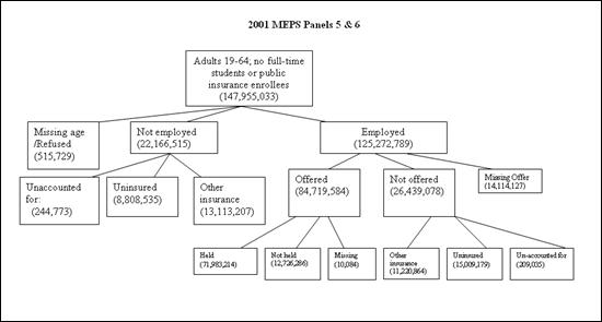
Figure A1 illustrates a diagram that depicts the age group of 19-64, this corresponds to 147,955,033 non-elderly adults in the United States. They are categorized into three different groups Missing age, Not employed and Employed. For this analysis, data from four large employers representing approximately 160,000 covered lives of information (including dependents) were available.
Consumer Directed Health Plan data (2001-2003):
The project investigators had access to de-identified data on the selection of health plans by employees, as well as their demographics. For this analysis, data from four large employers representing approximately 160,000 covered lives of information (including dependents) were available. Three of the four employers were national firms with substantial populations of employees; one was a large employer located in Minnesota. Each of these employers has offered a CDHP along with other traditional managed care plans. For the CDHP plans, each employer has received a take-up rate ranging between 4% and 15% in their first year offered.
Model Estimation
The model estimation had several steps. As a first step, we pooled the data from the three employers offering CDHPs to estimate a conditional logistic plan choice model similar to our earlier work (Parente, Feldman and Christianson, 2004). Conceptually, we used a choice model based on utility maximization, where utility is considered to be a function of personal attributes such as age, gender, income, chronic illness, and family status; health plan attributes such as the tax-adjusted, out-of-pocket premium and the deductible amount; and the interaction of personal and plan attributes. Personal characteristic variables were entered into the model as interactions of plan attribute variables. The coefficient estimates produced by this model represent the utility of each plan attribute to an employee.
In the second step we used the estimated choice-model coefficients to predict health plan choices for individuals in the MEPS-HC. In order to complete this step, it was necessary first to assign the number and types of health insurance choices that are available to each respondent in the MEPS-HC. For this purpose we turned to the smaller, but more-detailed MEPS Household
Component-Insurance Component linked file, which contained the needed information.
The steps taken to estimate this predictive model are highlighted in Figure 1. More detail of how these steps were executed is described below.
Estimate plan offerings using the MEPS linked data:
The MEPS "linked" Household Component-Insurance Component data file is a random sample of individuals who reported being employed and offered health insurance in Round 1 of the Household Component survey. These individuals were asked to provide contact information regarding their place of employment. Employers of these individuals were surveyed to provide detailed information about the number and types of plans that they offered to eligible workers. For each offered plan (up to four plans for private establishments and all plans for government organizations), an employer was asked to include the total premium, employee and employer shares of the total premium, and plan characteristics including hospital and physician coinsurance, hospital and physician copayments, and deductibles for individual and family coverage.
Since the linked sample only represents a subset of all offered workers in the Household
Component, we checked the representativeness of the linked sample using a binary logistic regression and found:
- Individuals in professional services and public administration were more likely to link than those in agriculture, mining, entertainment/recreation, personal services, and active military.
- Midwesterners were more likely to link relative to westerners.
- Whites were less likely to link relative to persons of "other" race.
- Government workers had a higher response rate than private-sector workers.
The link process was a function of the following variables: age, sex, race, marital status, dependents, geographic region, metropolitan (MSA) location, government employment, establishment size, industry category, wage income, and chronic illness (defined as a binary variable).
The linked data have 3,127 individuals and 7,802 plan-person observations. We do not have good information on response rates because we do not know what fraction of offered workers in MEPS was considered for the linked survey. In absolute terms, it appears that approximately 36% of offered workers linked.
Approximately 40% of linked workers have one plan offered to them, 19.7% have two plans offered, 11.8% have three plans, and the remaining 29.5% have four or more plans from which to choose. These percentages are not representative of the national proportions of workers who have one, two, three, and four or more plans offered to them because of the over-representation of government workers, who commonly have more offered plans than private-sector workers.
To predict the number and type of plans offered, we followed two steps:
1. Used the MEPS linked insurance file to estimate a model for the number and types of health plans offered to eligible workers (age 19-64, non public enrollees, non full-time students).
More specifically, we estimated an ordered probit model with the dependent variable taking the values of 1, 2, 3, or 4+ plans. The model included the following explanatory variables: age, male, white, black, marry, total number dependents, wage income, union member, works for government, establishment size, whether the establishment has more than one location, northeast, midwest, south, and MSA. The total number of observations was 2,891 and the R was .12.
2. Apply the model estimates to the MEPS-HC full sample to predict the number of plans for all respondents who were offered insurance by an employer.
Using the model estimates, for each individual who reported being offered employer group coverage in the MEPS-HC, we predicted the probability of each outcome (1, 2, 3, 4+ plans offered). We then identified the category that had the maximum probability among the four options.
We used a specific decision rule to assign the number of plans to each individual It included using both the category with the highest predicted probability as well as the individual's direct response to a question asked in the MEP-HC about whether he/she had a choice of plans. If he/she was reported not having a choice of plans, then the individual was assigned one plan. If he/she reported having plan choice, then the assigned number of plans reflected the outcome with the highest predicted probability among the 2, 3, and 4 plan options.
The types of plans were based on the distribution of plan offerings from the linked sample, conditional on the total number of plans offered. For example, individuals who had one plan offered to them were most likely to be offered a Preferred Provider Organization (PPO) plan.16 So, we assigned a PPO to those with one offered plan. The other assignments were as follows:
2 plans: PPO and HMO
3 plans: 2 PPOs and 1 HMO
4+ plans: 3 PPOs and 1 HMO
Estimate Premiums for Simulation:
One challenge we faced was how to designate specific plan attributes (e.g., coinsurance rate, deductible, etc.) for the assigned plan choices. Originally, we used summary statistics from the MEPS linked insurance file to identify the median characteristics of plans by type (PPO versus HMO) as well as coverage type (single versus family). To predict the premium that would be associated with a particular bundle of attributes, we estimated "hedonic" premium models. The specific equation used was:
Total premium = f(hospital coinsurance, physician coinsurance, and deductible).
The estimates for HMOs used patient co-payments (dollar payments per unit of service) rather than the physician coinsurance rate.
These equations were estimated separately by coverage type, plan type, and establishment size (e.g., single-coverage PPO offered by establishments with <50 workers). The model estimates were then used with the summary statistics to predict premiums for each plan, coverage type, and establishment size category (< 50; 50-200; >200) combination.
Finally, to obtain the employee's out-of-pocket premium cost, we multiplied predicted total premiums by the average proportion paid by employees for single and family coverage. We did not feel that the sample sizes were large enough reliably to perform this multiplication separately by coverage type and establishment size.
In our new approach, we used the claims data from the different health plan types to develop experience rated premiums for each person in the employer data using variables common to both the employer and MEPS database. We then computed group market community rated premiums for firms with different establishment sizes as was developed before. The key difference in the premium by establishment size was the loading factors we assumed which the smallest employers facing the highest loading charge and the largest employers facing the greatest loading charge. In the individual market, everyone faced their computed experience rated premium plus the smallest group loading charge.
Estimate Plan Choice Regression:
We pooled plan choice data from the four employers offering CDHPs to specify a conditional logistic regression model similar to our earlier work (Parente, Feldman and Christianson, 2004). Conceptually, we use a choice model based on utility maximization, where utility is considered to be a function of personal attributes such as health status, health plan attributes such as the out-of-pocket premium, and the interaction of premium and health status, formally stated as:
Uij = f(Zj,Yi,Xij)
Where i is the decision-making employee choosing among:
- j = health plan choices,
- Yi = employee personal attributes,
- Zj = health plan attributes and
- Xij = interactions between alternative-specific constants and personal attributes.
A very important constraint in our modeling was that any plan attribute used in the model from the employer data also had to be available in the MEPS data to permit a simulation. As a result, the key variables used in the plan choice model were:
- SCALEDPREM = After tax premium paid by the employee
- CLB = Amount of money in the employee’s health reimbursement account (HRA), if any.
- CUB = Difference between the employee’s plan deductible and the HRA.
- COIN = Coinsurance rate
- CHRONIC = Employee or dependent has a chronic illness=1, else 0 NEW
- AGE = Employee’s age (years)
- FEM = Employee’s gender (1=female, 0=male)
- FAM = Employee has a 2-person or family contract=1, else =0
- INC = Employee’s annual wage income.
Also included in the regression were alternative-specific constants (intercepts) for each of the possible health plan choices. These intercepts are used to capture plan-specific features not represented by other identifiers of plan design. They are also included as interaction terms with age, gender, family status and income. The intercept terms include:
- PPO_L = PPO Low (e.g., restrictive network, high co-pay, 15% coinsurance)
- PPO_M = PPO Medium (e.g., better network, lower co-pay and coinsurance)
- PPO_H = PPO High (e.g., open network, lowest co-pay, no coinsurance)
- HRA = Health Reimbursement Account CDHP
- HSA_E = Employer-sponsored HSA, modeled on higher premium cost HRA
- HSA_S = Employee-paid HSA, no employer contribution, modeled on lower premium cost HRA
- HMO = Health Maintenance Organization
Choice Set Assignment and Prediction
Assign Plan Choices to Full MEPS Sample:
We used the three data sources to develop two sets of plan choice predictions for the simulation: one set of data for workers with insurance offers and a second set for individuals who do not have employer offers of coverage. This second set includes both uninsured individuals, as well as those who take up non-group policies One group of individuals that we exclude from the simulation are non-offered individuals who reported having employer group coverage through another household member. Below we outline the analytic steps taken to develop the individuals' choice sets for the simulations.
1. Workers With Offers
We started with the original four choices predicted earlier, including three PPOs and an HMO. Since a worker was assigned between one and four plans, we needed to make some assumptions for each.
- 4 choices: Low PPO, Medium PPO, High PPO, HMO
- 3 choices: Low PPO, High PPO, HMO
- 2 choices: Medium PPO, HMO
- 1 choice: Medium PPO
Here, low, medium, and high refer to the cost and quality of the plans (e.g., low implies low cost and lower quality).
To these choices we added four additional options:
- Self-financed (full cost) HSA - Additional choice for all workers
- Turned down health coverage - Additional choice for all workers
- Employer sponsored HSA - Available to all workers in establishments with >500 employees, not available to other workers
- Employer sponsored HRA - Available to all workers in establishments with >500 employees, not available to other workers
2. Individuals Without an Insurance Offer
Individuals who did not have health insurance offered to them at work or who were not employed faced five health plan choices regardless of income, age or gender:
- High PPO
- Medium PPO
- Low PPO
- Self-financed HSA
- Uninsured
Use Parameter Estimates to Predict Plan Choice Probabilities:
With a total set of possible choices for workers with insurance offers and individuals without insurance offers, we used the plan choice regression results to predict plan choice probabilities
for each MEPS-HC sample respondent.17
However, before we could predict the probabilities, we needed to develop some specific assumptions about benefit plan design and premiums for individual plans. To get premium estimates, we originally used MEPS linked insurance data to develop a hedonic price model to predict premiums for individual plans. We worked with the same hedonic plan regressions described above, except that for individuals without offers of coverage, we used the premium model for the smallest establishment size category, based on the assumption that this most closely represents an individual policy in terms of the loading charge for plan administrative costs. The current approach used individual market premiums that were computed for each person in the MEPS plus a loading charge. The premium estimates came from health plan specific cost regressions. Originally, we needed to inflate premiums from 2001 prices to 2006 prices based medical insurance price inflation during the period. In the current model, we inflated the premiums from 2002 (the dominant year of the claims data used) to 2006.
The plan characteristics that we used to define the three PPOs (low, median, and high) came from the 2002 HIAA/eHealthinsurance.com survey of plans purchased in the individual market. Roughly speaking, we used the 25th, 50th, and 75th percentiles of coinsurance and deductibles for assigning the plan characteristics.
We also recognized that premiums in the individual market vary a lot by a person's age. The
MEPS survey included a table of average premiums by age cohort. Originally, we created an index using the information on this table. The index was set equal to 1.0 for the age group corresponding to the median age of adults in our sample (35-39). Older individuals, who had higher premiums, had index values that were greater than 1.0. Younger individuals, who had lower premiums, had index values less than 1.0. The index values ranged from .59 to 2.18 for single coverage policies and .453 to 1.65 for family coverage policies.
In the current model, we take age, gender, family contract and chronic illness into account to predict premiums used the health plans claims data. Finally, we adjusted all premiums to 2006 dollars.
Rescale Take-up Rates
One significant issue with our simulation is that we were not able to predict whether or not an individual would take-up insurance in the employer-offered market or be uninsured in the individual market. We faced this limitation because the CDHP employer data only includes information on offered workers who held coverage.
To address this issue, we needed to calibrate our model to accurately reflect both the actual percentage of people who turn down employer offers and the actual percentage of people in the individual market who are uninsured. To obtain more accurate estimates, we completed these calibrations by four quartiles of income and then compared our results to national, non-take-up and uninsurance rates. We also applied the national population weights to the calibrated model to represent the entire adult population, excluding full-time students, those with public insurance, and individuals with employer-based coverage through another household member. This fairly tedious process was performed for each re-estimation and/or modification of the conditional logistic regression.
Policy Simulation
To complete the simulations, two final steps remained. The first was to generate 2006 HSA
premiums and benefit designs. The second was to specify the various simulation proposals.
Define HSA Plan Design and Premium:
Starting in 2004, we assumed that all individuals in the non-group ("individual") market would have access to an HSA. We relied on the eHealthinsurance.com website (www.eHealthinsurance.com) for current information on HSA premiums and plan characteristics. We collected information on two HSA policies offered in the largest two cities across every state. Next, we estimated a hedonic premium equation that allowed us to predict the premium for different HSA designs. For all of the simulations, except one (described below), we used an HSA with a $1,000 spending account and a $3,500 deductible for single coverage and $2,000/$7,000 for families. The average monthly premium for our prototype HSA for a 40-year old non-smoking single male was $102.78 per month; for a 40-year old married male (also a non-smoker) with a spouse and two children under the age of ten, the monthly premium was $226.97.
This approach was the same we used in both simulations. The only difference was we updated the prices from 2005 to 2006 prices. When we completed a market scan of the same major markets examined before, we did not see many benefit design differences from the time of our original analysis.
The HSA premiums used in our simulations are the sum of the catastrophic policy price plus a $1,000 account. For example, a $6,500 HSA premium in our simulation for a family policy would be based on a $5,500 premium for a catastrophic insurance policy and a $1,000 HSA.
Benefit differences in HSAs can be large. For example, below we list two different HSA options,
a high a low deductible HSA plan in Santa Clara County, CA, that we found on eHealthinsurance.com in early, 2005:
HSA Option #1
Single Coverage:
- $1,000 HSA Account
- $3,500 Deductible
- $2,500 'Donut Hole' (DH starts at $1,001 of expenditure - ends at $3,500)
- 0% Coinsurance
- Premium includes catastrophic and $1,000 HSA Account.
- Thus, 100% catastrophic coverage starts at $3,501
Family Coverage:
- $1,000 HSA Account
- $7,000 Deductible
- $6,000 'Donut Hole' (DH starts at $1,001 of expenditure - ends at $7,000)
- 0% Coinsurance
- Premium includes catastrophic and $1,000 HSA Account.
- Thus, 100% catastrophic coverage starts at $7,001
HSA Option #2
Single Coverage:
- $1,000 HSA Account
- $2,600 Deductible
- $1,600 'Donut Hole' (DH starts at $1,001 of expenditure - ends at $2,600)
- 0% Coinsurance
- Premium includes catastrophic and $1,000 HSA Account.
Family Coverage:
- $1,000 HSA Account
- $2,600 Deductible
- $1,600 'Donut Hole' (DH starts at $1,001 of expenditure - ends at $2,600)
- 0% Coinsurance
- Premium includes catastrophic and $1,000 HSA Account.
HSA premiums were age-adjusted using the same method described above to rescale individual
PPO plan coverage. Note, the premiums used in the predictions included an annual payment of $1,000 into an HSA for both the single and family policies. We chose $1,000 because it was the lowest amount for a family coverage personal care account in our analysis of employer HRAs and a low to moderate amount for a single coverage personal care account.
Finally, it is important to note that for the Offered-turned down population, we have not explicitly taken account of whether these individuals have employer group coverage through another source (e.g., a working spouse). From the MEPS data, we do know that approximately 25% of those who turn down an offer of employer coverage are uninsured.
Also, in our take-up estimates, we have excluded all non-offered individuals who reported having employer group coverage from their partner through the offered-group market. This group represents approximately 29 million insured individuals.
Substantial Changes between the Original and Current Simulations
A. Variable Construction
The variables used in the simulation are: "SCLUB" = contribution to HSA based on age and income, "SCUB" = gap between contribution and HDHP deductible (which can be negative if
SCLUB exceeds the deductible), and "PREMIUM" = total premium. The total premium is equal to the insurance premium plus the tax-adjusted SCLUB. According to current law, tax deductibility of SCLUB is capped at $2,700 for single coverage and $5,450 for family coverage.
For example, suppose Joe is a single man in the 20% tax bracket who pays $1,500 for the insurance premium and makes a $3,760 annual HSA contribution. His PREMIUM = $1,500 +
($3,760 - $2,700) + $2,700 * (1 - .20) = $4,720.
B. 2006 State of the Union Simulation
The following example illustrates how the SOTU subsidies were simulated. Suppose Joe is eligible for a $500 low-income premium tax credit.18 After the credit, his net premium is $1,500 - $500 = $1,000. Assuming his income tax rate is 20 %, he receives an income tax deduction on the net premium of $1,000 * .20 = $200. He also receives an employment tax credit of $1,000 * .153 = $153. Joe's fully-adjusted insurance premium is therefore $1,500 - $500 - $200 - $153 = $647.
Joe also is able to increase his pre-tax HSA contribution to the out-of-pocket maximum of his insurance policy coverage, assumed to be $3,500 in our simulations. In effect, this provision makes all of Joe's out-of-pocket spending under the HDHP eligible for pre-tax status. In addition, individuals making after-tax HSA contributions would be allowed an employment tax credit on those contributions. In Joe's case, the two subsidies result in an after-tax HSA cost of ($3,760 - $3,500) * (1 - .153) + $3,500 * (1 -.20) = $3,020 (rounded to the nearest dollar). Therefore, Joe's total premium is $3,667.
C. Plan Choice Model
A multi-nominal logistic regression was used to create the plan choice estimates. These were all new estimates that included claims based measures of chronic illness. The plan choice equation applied to MEPS, along with the intercept terms for the turned down population and the uninsured, is presented in Table A1. The regression coefficients and tests of statistical significance are presented in Table A2.
D. Health Care Expenditures Model
Multivariate linear regression models were used to predict health plan expenditures by plan type.
The regression results to predict expenditures are presented in Tables A3 to A8.
Appendix A1: Plan Choice Regression Model (SAS Program Code)
LINR_PRED=
| (TAXADJPREM | * | -3.1796 | ) | + /* | Premium in (thousands) | */ | ||||||
| (SCLB | * | 2.39046 | ) | + /* | Account contribution (thousands) | */ | ||||||
| (SCUB | * | -1.62512 | ) | + /* | Deductible – account (thousands) | */ | ||||||
| (COINS | * | -16.2333 | ) | + /* | Coinsurance (0-1 | */ | ||||||
| (PPO_M_INT | * | 0.943117 | ) | + /* | PPO Medium intercept | */ | ||||||
| (PPO_H_INT | * | 1.31469 | ) | + /* | PPO High intercept | */ | ||||||
| (HRA_INT | * | -1.76626 | ) | + /* | HRA Intercept | */ | ||||||
| (HSA_S_INT | * | -2.80932 | ) | + /* | HSA Employer Provided Intercept | */ | ||||||
| (HSA_E_INT | * | -2.80932 | ) | + /* | HSA opt-out/ Individual Intercept | */ | ||||||
| (HMO_INT | * | 2.44818 | ) | + /* | HMO Intercept | */ | ||||||
| ((faMPRMI | * | 1.83379 | ) | + /* | Family Contract (0,1) * Premium | */ | ||||||
| ((PPO_M_INT*sAGE | * | -1.56416 | ) | + /* | PPO MediuM Age (in hundreds) | */ | ||||||
| ((PPO_H_INT*sAGE | * | -1.75401 | ) | + /* | PPO High * Age (in hundreds | */ | ||||||
| ((HRA_INT *sAGE | * | -2.34963 | ) | + /* | HRA * Age (in hundreds) | */ | ||||||
| ((HSA_S_INT*sAGE | * | -1.99124 | ) | + /* | HSA EmployeRAge (in hundreds) | */ | ||||||
| ((HSA_E_INT*sAGE | * | -1.99124 | ) | + /* | HSA Individual * Age (hundreds | */ | ||||||
| ((HMO_INT *sAGE | * | -4.20002 | ) | + /* | HMO * Age (in hundreds) | */ | ||||||
| ((PPO_M_INT*INC | * | -0.00473388 | ) | + /* | PPO MediuM Income (thousands) | */ | ||||||
| ((PPO_H_INT*INC | * | -0.00452832 | ) | + /* | PPO High * Income (thousands) | */ | ||||||
| ((HRA_INT *INC | * | 0.00567068 | ) | + /* | HRA * Income (thousands) | */ | ||||||
| ((HSA_S_INT*INC | * | 0.00480442 | ) | + /* | HSA EmployeRIncome (thousands) | */ | ||||||
| ((HSA_E_INT*INC | * | 0.00480442 | ) | + /* | HSA Individual* Income(thousands) | */ | ||||||
| ((HMO_INT *INC | * | -0.00860868 | ) | + /* | HMO * Income (thousands) | */ | ||||||
| ((PPO_M_INT*FEM | * | 0.419878 | ) | + /* | PPO MediuM Female | */ | ||||||
| ((PPO_H_INT*FEM | * | 0.332876 | ) | + /* | PPO High * Female | */ | ||||||
| ((HRA_INT *FEM | * | 0.108911 | ) | + /* | HRA * Female | */ | ||||||
| ((HSA_S_INT*FEM | * | 0.267474 | ) | + /* | HSA EmployeRFemale | */ | ||||||
| ((HSA_E_INT*FEM | * | 0.267474 | ) | + /* | HSA Individual* Female | */ | ||||||
| ((HMO_INT* FEM | * | 0.0396604 | ) | + /* | HMO * Female | */ | ||||||
| ((PPO_M_INT*FAM | * | -0.423343 | ) | + /* | PPO MediuM Family (0,1) | */ | ||||||
| ((PPO_H_INT*FAM | * | -0.200933 | ) | + /* | PPO High * Family | */ | ||||||
| ((HRA_INT *FAM | * | 0.0239377 | ) | + /* | HRA * Family | */ | ||||||
| ((HSA_S_INT*FAM | * | 1.11915 | ) | + /* | HSA EmployeRFamily | */ | ||||||
| ((HSA_E_INT*FAM | * | 1.11915 | ) | + /* | HSA Individual* Family | */ | ||||||
| ((HMO_INT *FAM | * | -0.99562 | ) | + /* | HMO * Family | */ | ||||||
| ((PPO_M_INT*CHR | * | 0.275686 | ) | + /* | PPO MediuM Chronic (0,1) | */ | ||||||
| ((PPO_H_INT*CHR | * | 1.18185 | ) | + /* | PPO High * Chronic (0,1) | */ | ||||||
| ((HRA_INT *CHR | * | 0.771403 | ) | + /* | HRA * Chronic (0,1) | */ | ||||||
| ((HSA_S_INT*CHR | * | 0.680646 | ) | + /* | HSA EmployeRChronic (0,1) | */ | ||||||
| ((HSA_E_INT*CHR | * | 0.680646 | ) | + /* | HSA Individual* Chronic (0,1) | */ | ||||||
| ((HMO_INT *CHR | * | 0.516199 | ) | + /* | HMO * Chronic (0,1) | */ | ||||||
| ((TAXADJPREMCHR | * | -0.332006 | ) | + /* | PremiuM Chronic (0,1) | */ | ||||||
| ((SCLB *CHR | * | -0.275012 | ) | + /* | Account * Chronic | */ | ||||||
| ((SCUB *CHR | * | -0.381562 | ) | + /* | Deductible_Account Gap *Chronic | */ | ||||||
| ((COINS *CHR | * | -2.06644 | ) | + /* | CoinsurancE Chronic | */ | ||||||
| ((SCLB *FAM | * | -1.93489 | ) | + /* | Account * Family | */ | ||||||
| ((SCUB *FAM | * | 0.675129 | ) | + /* | Deductible_Account Gap * Family | */ | ||||||
- Pchoice = Plan Choice (in text);
- Wagepinc = Wages from MEPS Data;
| if PCHOICE='UNINS' then do; | |||||
| if wagepinc<=15050 | then do; linr_pred=-9.70 | ; | INC_QUAT='1 - <50th' | ; | end; |
| if 15050<wagepinc<=25078 | then do; linr_pred=-10.3 | ; | INC_QUAT='3 - 50-75th' | ; | end; |
| if wagepinc>25078 | then do; linr_pred=-11.35 | ; | INC_QUAT='4 - >75th ' | ; | end; |
| end; | |||||
| if PCHOICE='TURND' then do; | |||||
| if wagepinc<=9378 | then do; linr_pred=-4.7 | ; | INC_QUAT='1 - <25th' | ; | end; |
| if 9378<wagepinc<=24500 | then do; linr_pred=-4.9 | ; | INC_QUAT='2 - 25-50th' | ; | end; |
| if 24500<wagepinc<=41288 | then do; linr_pred=-5.5 | ; | INC_QUAT='3 - 50-75th' | ; | end; |
| if wagepinc>41288 | then do; linr_pred=-5.95 | ; | INC_QUAT='4 - >75th | ; | end; |
| end; | |||||
exppred=exp(LINR_PRED);
run;
Appendix A2: Plan Choice Regression Results
Variable Definition from SAS program in Appendix A1
| Data Output from LIMDEP | ||
|---|---|---|
| --> | namelist ; x2 = SCMEDPR2,SCLB,SCUB , COINS, | |
| PPO2,PPO1,DEF1, DEF3, HMO1,FAM_PREM, | ||
| PPO2_AGE,PPO1_AGE,DEF1_AGE,DEF3_AGE,HMO1_AGE, | ||
| PPO2_INC,PPO1_INC,DEF1_INC,DEF3_INC,HMO1_INC, | ||
| PPO2_FEM,PPO1_FEM,DEF1_FEM,DEF3_FEM,HMO1_FEM, | ||
| PPO2_FAM,PPO1_FAM,DEF1_FAM,DEF3_FAM,HMO1_FAM, | ||
| PPO2_CHR,PPO1_CHR,DEF1_CHR,DEF3_CHR,HMO1_CHR, | ||
| CHR_PREM,CHR_SCLB,CHR_SCUB,CHR_COIN,FAM_SCLB,FAM_SCUB $ | ||
| --> | DISC;Lhs=yvar, CHOICES; Rhs=x2 | |
| ;Choices = P1,P2,P3,D1,D3,H1 $ | ||
| Normal exit from iterations. Exit status=0. | ||
| Discrete choice (multinomial logit) model | |||
|---|---|---|---|
| Maximum Likelihood Estimates | |||
| Dependent variable | Choice | ||
| Weighting variable | ONE | ||
| Number of observations | 26734 | ||
| Iterations completed | 8 | ||
| Log likelihood function | -27200.62 | ||
| Log-L for Choice | model = | -27200.6225 | |
| R2=1-LogL/LogL* | Log-L fncn | R-sqrd | RsqAdj |
| No coefficients | -47900.8977 | .43215 | .43192 |
| Constants only. | Must be computed directly. | ||
| Use NLOGIT ;...; RHS=ONE $ | |||
| Response data are given as ind. choice. | |||
| Number of obs.= 26978, skipped 244 bad obs. | |||
| Variable | Coefficient | Standard Error | b/St.Er. | P[|Z|>z] | Mean of X |
|---|---|---|---|---|---|
| SCMEDPR2 | -3.179598898 | .13294966 | -23.916 | .0000 | |
| SCLB | 2.390461410 | .27043780 | 8.839 | .0000 | |
| SCUB | -1.625123020 | .71731108E-01 | -22.656 | .0000 | |
| COINS | -16.23330404 | .73243997 | -22.163 | .0000 | |
| PPO2 | .9431168496 | .13457443 | 7.008 | .0000 | |
| PPO1 | 1.314687513 | .14143793 | 9.295 | .0000 | |
| DEF1 | -1.766260950 | .22458990 | -7.864 | .0000 | |
| DEF3 | -2.809316873 | .24690227 | -11.378 | .0000 | |
| HMO1 | 2.448179610 | .16031190 | 15.271 | .0000 | |
| FAM_PREM | 1.833787851 | .14095827 | 13.009 | .0000 | |
| PPO2_AGE | -1.564161860 | .30350630 | -5.154 | .0000 | |
| PPO1_AGE | -1.754006739 | .30828143 | -5.690 | .0000 | |
| DEF1_AGE | -2.349634141 | .43953766 | -5.346 | .0000 | |
| DEF3_AGE | -1.991238499 | .36560470 | -5.446 | .0000 | |
| HMO1_AGE | -4.200015687 | .34344449 | -12.229 | .0000 | |
| PPO2_INC | -.4733881586E-02 | .14444996E-02 | -3.277 | .0010 | |
| PPO1_INC | -.4528320996E-02 | .14534194E-02 | -3.116 | .0018 | |
| DEF1_INC | .5670676142E-02 | .15519452E-02 | 3.654 | .0003 | |
| DEF3_INC | .4804414933E-02 | .14601218E-02 | 3.290 | .0010 | |
| HMO1_INC | -.8608681275E-02 | .15586591E-02 | -5.523 | .0000 | |
| PPO2_FEM | .4198777835 | .64038275E-01 | 6.557 | 0000 | |
| PPO1_FEM | .3328763673 | .64646458E-01 | 5.149 | 0000 | |
| DEF1_FEM | .1089110668 | .92207787E-01 | 1.181 | .2375 | |
| DEF3_FEM | .2674740899 | .75607620E-01 | 3.538 | .0004 | |
| HMO1_FEM | .3966044321E-01 | .73044431E-01 | .543 | .5872 | |
| PPO2_FAM | -.4233426685 | .70287922E-01 | -6.023 | .0000 | |
| PPO1_FAM | -.2009330220 | .93664020E-01 | -2.145 | .0319 | |
| DEF1_FAM | .2393773926E-01 | .16172454 | .148 | .8823 | |
| DEF3_FAM | 1.119148744 | .24404543 | 4.586 | .0000 | |
| HMO1_FAM | -.9956198572 | .88505887E-01 | -11.249 | .0000 | |
| PPO2_CHR | .2756860412 | .73561832E-01 | 3.748 | .0002 | |
| PPO1_CHR | 1.181854939 | .90345940E-01 | 13.081 | .0000 | |
| DEF1_CHR | .7714034791 | .12725272 | 6.062 | .0000 | |
| DEF3_CHR | .6806458551 | .15519146 | 4.386 | .0000 | |
| HMO1_CHR | .5161991059 | .85864350E-01 | 6.012 | .0000 | |
| CHR_PREM | -.3320055569 | .72412958E-01 | -4.585 | .0000 | |
| CHR_SCLB | -.2750123438 | .10215671 | -2.692 | .0071 | |
| CHR_SCUB | -.3815617266 | .51005777E-01 | -7.481 | .0000 | |
| CHR_COIN | -2.066440812 | .95041146 | -2.174 | .0297 | |
| FAM_SCLB | -1.934888084 | .25901932 | -7.470 | .0000 | |
| FAM_SCUB | .6751292839 | .75349008E-01 | 8.960 | .0000 |
Appendix A3 – HMO Health Care Expenditure Model (SAS Output)
| DF | Mean Square | F Value | Pr > F | |||
|---|---|---|---|---|---|---|
| Model | 5 | 29864081711 | 157.53 | <.0001 | ||
| Error | 9076 | 189575329 | ||||
| Corrected Total | 9081 | |||||
| Root MSE | R-Square | 0.0799 | ||||
| Dependent Mean | Adj R-Sq | 0.0793 | ||||
| Coeff Var | ||||||
| Variable | DF | Parameter Estimate |
Standard Error | t Value | Pr > |t| |
|---|---|---|---|---|---|
| Intercept | 1 | -2588.77928 | 576.28374 | -4.49 | <.0001 |
| Female (=1) | 1 | 4.20294 | 301.71728 | 0.01 | 0.9889 |
| Income ('000s) | 1 | -10.64084 | 6.24156 | -1.70 | 0.0883 |
| Age ('00s) | 1 | 9162.01982 | 1415.10020 | 6.47 | <.0001 |
| Family=1 | 1 | 3655.77272 | 312.88459 | 11.68 | <.0001 |
| Chronic Ill=1 | 1 | 5385.49451 | 317.12188 | 16.98 | <.0001 |
Appendix A4 – Low Option HRA Health Care Expenditure Model (SAS Output)
| Source | DF | Sum of Squares | Mean Square | F Value | Pr > F |
|---|---|---|---|---|---|
| Model | 7 | 2020674807 | 288667830 | 6.66 | <.0001 |
| Error | 807 | 35000952186 | 43371688 | ||
| Corrected Total | 814 | 37021626992 | |||
| Root MSE | 6585.71848 | R-Square | 0.0546 | ||
| Dependent Mean | 2156.38643 | Adj R-Sq | 0.0464 | ||
| Coeff Var | 305.40530 |
| Variable | DF | Parameter Estimate |
Standard Error | t Value | Pr > |t| |
|---|---|---|---|---|---|
| Intercept | 1 | -1484.23490 | 1211.94364 | -1.22 | 0.2211 |
| Female (=1) | 1 | -401.23975 | 473.21169 | -0.85 | 0.3967 |
| Income ('000s) | 1 | 1.33132 | 6.18639 | 0.22 | 0.8297 |
| Age ('00s) | 1 | 6067.52791 | 2339.83860 | 2.59 | 0.0097 |
| Family=1 | 1 | -12.14860 | 518.34404 | -0.02 | 0.9813 |
| Chronic Ill=1 | 1 | 2449.72600 | 492.02318 | 4.98 | <.0001 |
| Deductible($) | 1 | -97.52082 | 261.12087 | -0.37 | 0.7089 |
| Coinsurance(%) | 1 | 3109.14987 | 2864.23170 | 1.09 | 0.2780 |
Appendix A5 – High Option HRA Health Care Expenditure Model (SAS Output)
| Source | DF | Sum of Squares | Mean Square | F Value | Pr > F |
|---|---|---|---|---|---|
| Model | 7 | 38203660292 | 5457665756 | 36.79 | <.0001 |
| Error | 2693 | 3.994551E11 | 148330890 | ||
| Corrected Total | 2700 | 4.376587E11 | |||
| Root MSE | 12179 | R-Square | 0.0873 | ||
| Dependent Mean | 5648.66650 | Adj R-Sq | 0.0849 | ||
| Coeff Var | 215.61048 |
| Variable | DF | Parameter Estimate |
Standard Error | t Value | Pr > |t| |
|---|---|---|---|---|---|
| Intercept | 1 | -818.06484 | 1102.44013 | -0.74 | 0.4581 |
| Female (=1) | 1 | -71.19379 | 508.34685 | -0.14 | 0.8886 |
| Income ('000s) | 1 | 8.67475 | 3.37356 | 2.57 | 0.0102 |
| Age ('00s) | 1 | 5546.76135 | 2605.39887 | 2.13 | 0.0333 |
| Family=1 | 1 | 3193.90066 | 660.60306 | 4.83 | <.0001 |
| Chronic Ill=1 | 1 | 5362.45013 | 513.94063 | 10.43 | <.0001 |
| Deductible($) | 1 | -1714.22917 | 784.88686 | -2.18 | 0.0290 |
| Coinsurance(%) | 1 | -4818.15443 | 4790.71208 | -1.01 | 0.3146 |
Appendix A6 – High Option PPO Health Care Expenditure Model (SAS Output)
| Source | DF | Sum of Squares | Mean Square | F Value | Pr > F |
|---|---|---|---|---|---|
| Model | 7 | 74729335548 | 10675619364 | 27.39 | <.0001 |
| Error | 4192 | 1.634048E12 | 389801466 | ||
| Corrected Total | 4199 | 1.708777E12 | |||
| Root MSE | 19743 | R-Square | 0.0437 | ||
| Dependent Mean | 4083.09431 | Adj R-Sq | 0.0421 | ||
| Coeff Var | 483.53991 |
| Variable | DF | Parameter Estimate |
Standard Error | t Value | Pr > |t| |
|---|---|---|---|---|---|
| Intercept | 1 | 2980.62690 | 1466.91736 | 2.03 | 0.0422 |
| Female (=1) | 1 | -290.30650 | 411.06713 | -0.71 | 0.4801 |
| Income ('000s) | 1 | -7.30764 | 6.02970 | -1.21 | 0.2256 |
| Age ('00s) | 1 | 4164.74362 | 1939.08087 | 2.15 | 0.0318 |
| Family=1 | 1 | 1144.35128 | 625.25338 | 1.83 | 0.0673 |
| Chronic Ill=1 | 1 | 3218.41265 | 465.66603 | 6.91 | <.0001 |
| Deductible($) | 1 | 4284.96265 | 1153.78112 | 3.71 | 0.0002 |
| Coinsurance(%) | 1 | -30035 | 7879.04311 | -3.81 | 0.0001 |
Appendix A7 – Medium Option PPO Health Care Expenditure Model (SAS Output)
| Source | DF | Sum of Squares | Mean Square | F Value | Pr > F |
|---|---|---|---|---|---|
| Model | 7 | 1.647226E11 | 23531800947 | 110.31 | <.0001 |
| Error | 8036 | 1.714312E12 | 213329057 | ||
| Corrected Total | 8043 | 1.879035E12 | |||
| Root MSE | 14606 | R-Square | 0.0877 | ||
| Dependent Mean | 3729.38308 | Adj R-Sq | 0.0869 | ||
| Coeff Var | 391.64087 |
| Variable | DF | Parameter Estimate |
Standard Error | t Value | Pr > |t| |
|---|---|---|---|---|---|
| Intercept | 1 | 587.12370 | 977.23878 | 0.60 | 0.5480 |
| Female (=1) | 1 | -253.20110 | 270.02291 | -0.94 | 0.3484 |
| Income ('000s) | 1 | -2.52179 | 4.45995 | -0.57 | 0.5718 |
| Age ('00s) | 1 | 3655.94155 | 1363.58034 | 2.68 | 0.0074 |
| Family=1 | 1 | 1822.27673 | 357.54176 | 5.10 | <.0001 |
| Chronic Ill=1 | 1 | 5296.90360 | 289.94977 | 18.27 | <.0001 |
| Deductible($) | 1 | -2098.66733 | 472.75382 | -4.44 | <.0001 |
| Coinsurance(%) | 1 | 428.86112 | 6043.31106 | 0.07 | 0.9434 |
Appendix A8 – Low Option PPO Health Care Expenditure Model (SAS Output)
| Source | DF | Sum of Squares | Mean Square | F Value | Pr > F |
|---|---|---|---|---|---|
| Model | 5 | 29535932372 | 5907186474 | 14.60 | <.0001 |
| Error | 1655 | 6.697573E11 | 404687186 | ||
| Corrected Total | 1660 | 6.992932E11 | |||
| Root MSE | 20117 | R-Square | 0.0422 | ||
| Dependent Mean | 2992.90458 | Adj R-Sq | 0.0393 | ||
| Coeff Var | 672.15101 |
| Variable | DF | Parameter Estimate |
Standard Error | t Value | Pr > |t| |
|---|---|---|---|---|---|
| Intercept | 1 | -2474.05250 | 1251.44180 | -1.98 | 0.0482 |
| Female (=1) | 1 | -110.94744 | 556.83431 | -0.20 | 0.8421 |
| Income ('000s) | 1 | 4.50862 | 10.58875 | 0.43 | 0.6703 |
| Age ('00s) | 1 | 5416.31686 | 2884.28544 | 1.88 | 0.0606 |
| Family=1 | 1 | 2222.38383 | 605.90688 | 3.67 | 0.0003 |
| Chronic Ill=1 | 1 | 3303.98688 | 585.00965 | 5.65 | <.0001 |
Footnotes
1 2006 Blue Book, United States Department of the Treasury, February, 2006.
2 HDHP stands for High Deductible Health Plan. This plan design generally has a substantial deductible and/or coinsurance requirement that must be met before catastrophic health insurance is activated for medical care reimbursement.
3 Stephen T. Parente, Roger Feldman, Jon B. Christianson, and Jean Abraham, Health Savings Accounts: Early Estimations on National Take-up from 2003 MMA and Future Policy Proposals, Final Report on Contract HHSP233200400573P: Analytic Support in Assessing the Impact of Health Savings Accounts on Health Insurance Coverage and Costs, June 7, 2005. Also see Roger Feldman, Stephen T. Parente, Jean Abraham, Jon B. Christianson, and Ruth Taylor, "Health Savings Accounts: Early Evidence of National Take-up from the 2003 Medicare Modernization Act and Future Policy Proposals," Health Affairs, 24:6 (November/December, 2005), pp. 1582-1591.
4 We modeled the tax credit based on the U.S. Department of the Treasury Blue Book published in February, 2004. Specifically, we used $1,000 and $556 tax credits with incomes at $15,000 and $20,000 respectively. No tax credit applied once income was at $30,000. These parameters were used to develop ratios to permit a sliding scale of tax credits with two kinks at $15,001 and $20,001. We also modeled the tax credit applying to dependents (starting at $500) at higher income breaks associated with families.
5 U.S. Treasury Department, General Explanations of the Administration's Fiscal Year 2007 Revenue Proposals ("2006 Blue Book"), February 6, 2006, available for viewing at http://www.treasury.gov/offices/tax-policy.
6 As a sensitivity test we added the average state rate to the tax subsidy, weighted by the number of people living in a state. We did not find any substantial difference in the distribution of the resulting plan choices in the simulation.
7 The proportion of the population for whom the cap on the tax subsidy was binding was very small, less than 5%. At one point we changed the age/income-specific contributions to the HSA just to make sure the cap might affect someone in the simulation.
8 Weiner J, Starfield B, Steinwachs D, and Mumford L. Development and Application of a Population Oriented Measure of Ambulatory Care Case-Mix. Med Care 1991;29:452-472.
9 As part of the calibration, we sought to have our estimated take-up be in the ball-park of the original analysis. However, we did not constrain the model to be exactly the same. As part of several additional sensitivity tests we used our old model with new data and the found the results to be similar. Some new employer data did change the results because of the use of their claims data and their very low use, given their age and gender profile. Tables with previous sensitivity analyses are available upon request.
10 Mark Pauly and Bradley Herring (Pooling Health Insurance Risks, Washington, DC: The AEI Press, 1999) have suggested that individual policies contain some degree of group experience rating and vice versa. According to Pauly and Herring, premiums in the individual market don’t rise one-for-one with predictable expenses, and premiums in the ESI market have a positive association with predicted individual medical expenditures, contrary to the GER hypothesis. Notwithstanding these findings, we decided to use IER and GER as our rating assumptions because these methods are more tractable and because it is not clear how to combine them to form “mixed” ratings systems as suggested by Pauly and Herring.
11 See Mark Pauly, Allison Percy, and Bradley Herring, “Individual Versus Job-Based Health Insurance: Weighing the Pos and Cons,” Health Affairs, 18:6 ((November/December, 1999), pp. 28-44 for data on loading fees in the individual health insurance market.
12 The MEPS uses "establishment size" rather than employer size. The three size classes are fewer than 50 employees, 50-200, and more than 200. We assume the loading factors for these classes are 20%, 15%, and 10% respectively.
13 We used rule (1) - the refundable tax credit equals 15.3 % of the HDHP premium - in all cases because most taxpayers have employment-taxable wages that exceed the HDHP premium.
14 We assume that employees as a group pay for health insurance through lower wages. Consequently, even if the individual's wage does not increase when he/she drops ESI, wages for the group increase and the government collects more income and employment taxes. For empirical evidence that workers bear the full incidence of health insurance benefits, see Jonathan Gruber, "The Incidence of Mandated Maternity Benefits," American Economic Review, 84:3 (June, 1994), pp. 622-641; and Jonathan Gruber and Alan Krueger, "The Incidence of Mandated Employer-Provided Insurance: Lessons from Workers' Compensation Insurance," in Tax Policy and the Economy, MIT Press for the National Bureau of Economic Research, 1991, pp. 111-143.
15 Estimates of previous premium elasticities are available from our 2005 NBER working paper presentation at the www.ehealthplan.org web site.
16 MEPS follows the unconventional notation of "Mixed" provider organization for PPO, "Exclusive" provider organization for HMO, and "Any" provider organization for conventional open access fee-for-service plan. Relatively few of the latter plans were represented in the data; therefore we did not assign a conventional plan to any worker with an employment-based offer.
17 We converted HMO co-pays to actuarially-equivalent coinsurance rates for predicting the HMO enrollment probability.
18 "Joe" doesn't really exist as a unique person because only high-income taxpayers contribute $3,760 to their HSA and only low-income taxpayers are eligible for a premium tax credit. Our hypothetical example combines several people to illustrate how all the subsidies were calculated.