
U.S. Department of Health and Human Services
A National Study of Assisted Living for the Frail Elderly: Final Sampling and Weighting Report
Vincent Iannacchione, Margaret Byron, Linda Lux and Lisa WrageResearch Triangle Institute
Catherine HawesMyers Research Institute
March 10, 1999
PDF Version: http://aspe.hhs.gov/daltcp/reports/sampweig.pdf (38 PDF pages)
This report was prepared under contracts #HHS-100-94-0024 and #HHS-100-98-0013 between the U.S. Department of Health and Human Services (HHS), Office of Disability, Aging and Long-Term Care Policy (DALTCP) and and the Research Triangle Institute. Additional funding was provided by American Association of Retired Persons, the Administration on Aging, the National Institute on Aging, and the Alzheimers Association. For additional information about this subject, you can visit the DALTCP home page at http://aspe.hhs.gov/_/office_specific/daltcp.cfm or contact the ASPE Project Officer, Gavin Kennedy, at HHS/ASPE/DALTCP, Room 424E, H.H. Humphrey Building, 200 Independence Avenue, S.W., Washington, D.C. 20201. His e-mail address is: Gavin.Kennedy@hhs.gov.
The opinions and views expressed in this report are those of the authors. They do not necessarily reflect the views of the Department of Health and Human Services, the contractor or any other funding organization.
TABLE OF CONTENTS
- 3. SAMPLING WEIGHTS FOR FACILITIES, RESIDENTS AND STAFF MEMBERS
- 3.1 Facility Screening Weights
- 3.2 Tier #3 and Tier #3 Facility Weights
- 3.3 Resident and Staff Member Weights
- APPENDIX A: CLASSIFICATION OF FACILITIES WITH MISSING OR CONFLICTING DATA
- LIST OF TABLES
- TABLE 1: Tier Classification of Survey-Eligible Facilities by Level of Privacy and Level of Service
- TABLE 2: Summary of the Sampling Design
- TABLE 3: Comparison of the State-Level Distribution of FSUs for Two Size Measures: Population 65 & Over versus Estimated Number of Candidate ALFs
- TABLE 4: Distribution of Candidate ALFs by Source Listing
- TABLE 5: Distribution of Candidate ALFs by Number of Source Listings and Size Category
- TABLE 6: Estimated Size Distribution of Candidate ALFs with Unknown Capacities
- TABLE 7: Cost Factors by Size Category
- TABLE 8: Distribution of Eligible Facilities by Level of Privacy and Service
- TABLE 9: Distribution of Tier #2 and Tier #3 Facilities Located in the 40-FSU Subsample
- TABLE 10: Final Disposition of the Facility Screening Sample
- TABLE 11: Estimated National Distribution of Eligible Facilities by Privacy and Service Levels
- TABLE 12: Expected Detectable Differences for Comparing Percentage Estimates between Tier #1, #2 and #3 Facilities Identified during the Facility Screening
- TABLE 13: Distribution of Questionnaires Obtained from Eligible Tier #3 Facilities
- TABLE 14: Tier #2 and Tier #3 Facility-Level Response Rates
- TABLE 15: Expected Detectable Differences for Comparing Percentage Estimates between Tier #2 and Tier #3 Facilities with Various Combinations of Privacy and Service
- TABLE 16: Staff Member Response Rates in Participating Tier #3 Facilities
- TABLE 17: Resident Response Rates in Participating Tier #3 Facilities
1. TARGET POPULATION
The target population for the National Study of Assisted Living for the Frail Elderly encompassed eligible assisted living facilities (ALFs) with eleven or more beds operating in the United States at the time of screening and data collection (Spring and Summer, 1998), as well as their operators, residents, staff members, and families of residents. To be eligible, an ALF had to be:
- a "self-proclaimed" facility that advertises or calls itself assisted living, serves the elderly and has 11 or more beds; and/or,
- an "otherwise nominated" facility that has 11 or more beds, serves the elderly, and provides (or arranges) meals, 24-hour staff, housekeeping, and assistance with at least two activities of daily living (ADLs) (which includes medication administration or assistance with self-administered medications).
The study excludes facilities with 10 or fewer beds for three reasons. First, we expect most of these facilities to be board and care homes which do not provide the level of care and services commonly associated with assisted living. Data from the 1993 ASPE Board and Care Study (Hawes et al., 1995a) and a study of a probability sample of domiciliary care home residents in North Carolina (Hawes et al., 1995b) show that very small facilities are more likely than larger homes to serve a younger population with developmental disabilities or chronic mental illness. They are also less likely to make a wide array of services available to residents, and much less likely to have a nurse on staff. Thus, including them on the sampling frame would have contributed to a large number of ineligible facilities being found during the screening calls. Second, in practice, few places with fewer than 11 beds refer to themselves as assisted living. For example, in Oregon, which has a specific "assisted living" licensure category and which allows licensure of places with fewer than 10 beds, no facilities that small have been constructed. Thus, we believe it is unlikely that otherwise eligible facilities will be eliminated simply because of size criterion. Third, including the small homes would mean basically re-examining many issues that were addressed in the ASPE Board and Care Study and would, in many ways, duplicate that effort.
We also excluded those facilities that do not serve the elderly; those licensed for only special populations (e.g., persons with developmental disabilities); and those licensed only as nursing homes (although places with nursing homes and other residential settings may be eligible).
The target population is divided into the three sub-populations or tiers shown in Table 1. Tier membership is defined by the combined level of services and privacy offered by a survey-eligible facility. During the design phase of the study, we developed working definitions for each of the levels of service and privacy. The working definitions were modified based on the results of the facility screening survey and are listed below.
| TABLE 1. Tier Classification of Survey-Eligible Facilities by Level of Privacy and Level of Service | |||
| Level of Service | Level of Privacy | ||
| High | Low | Minimal | |
| High | Tier #3 | Tier #3 | Tier #1 |
| Low | Tier #3 | Tier #2 | Tier #1 |
| Minimal | Tier #1 | Tier #1 | Tier #1 |
Levels of Service. We classified a survey-eligible facility as offering High Service if it provides or arranges the following services:
- Two meals a day;
- Housekeeping;
- 24-hour staff oversight; and
- Assistance with medications and at least one ADL or assistance with two or more ADLs;
In addition, it should:
- Provide (not just arrange) nursing care or monitoring as needed; and
- Have a full-time RN on staff.
Survey-eligible facilities that provide or arrange all but the last service were classified as offering Low Service. We classified all other survey-eligible facilities as offering Minimal Service.1
Levels of Privacy. We classified a survey-eligible facility as offering High Privacy if:
- None of its apartments or bedrooms house more than two unrelated residents; and,
- At least 80 percent of its apartments or bedrooms are private.
Survey-eligible facilities that satisfy only the first requirement were classified as offering Low Privacy and facilities that satisfy neither requirement were classified as offering Minimal Privacy.1
Tier #1 facilities offer either Minimal Service and/or Minimal Privacy and were not subject to further data collection beyond the facility screening activity.
Tier #2 facilities offer Low Service and Low Privacy and were surveyed by telephone with the Operator Telephone Interview and asked questions about their ownership, size, length of time in operation, staffing, specific services provided, and resident mix.
Tier #3 facilities offer either High Service and Low Privacy, Low Service and High Privacy, or High Service and High Privacy. Tier #3 facilities were surveyed with the Operator In-Person Interview, and the Operator Self-Administered Supplemental Questionnaire. Also, we conducted a structured observation of the Tier #3 facilities using the Walk-Through Observation instrument. Thus, for these facilities, there is very detailed information about resident case mix, services, rates, admission and discharge policies, visiting hours, other policies related to resident autonomy, operator background, staff training, facility ownership, and affiliations with multi-facility systems.
In addition, a probability sample of staff and residents of Tier #3 facilities were interviewed on-site, using the Staff Member Interview and the Resident Interview. If members of the resident sample were cognitively impaired or physically unable to participate, proxy respondents were identified. For each resident requiring a proxy, we used the Resident Proxy Respondent Interview to interview a staff member who provided him or her with direct care. We also interviewed a family member of residents who required a proxy using the Family Member Telephone Interview. Finally, members of the resident sample in the Tier #3 facilities who are discharged, die or otherwise exit the facility within the first six months following the site visit will be interviewed, using either the Discharged Resident Telephone Interview or Discharged Resident Proxy Respondent Telephone Interview. The documentation of the Discharged Resident Survey will be provided under separate cover.
2. SAMPLING DESIGN
The sampling design may be summarized as a stratified, three-stage, national probability sample with the following sampling units defined at each stage:
First-Stage Sampling Units (FSUs): Counties or county equivalents;
Second-Stage Sampling Units: Geographic addresses within selected FSUs that contain one or more candidate ALFs;2 and,
Third-Stage Sampling Units: Residents, their family members, and staff members of selected Tier #3 ALFs.
Because much of the sampling variance associated with planned population estimates is expected to be attributable to differences among facilities, we used epsem (equal probability of selection method) (see Kish, 1965, p.21) to achieve (to the extent possible) a self-weighting sample of survey-eligible facilities within each stratum. Self-weighting (a.k.a. equal weighting) samples reduce design effects because equal selection probabilities are assigned to all members of a population or stratum. The stratification and sample allocation for each stage of sampling are presented in Table 2.
First-Stage Sample of Counties. Unlike nursing homes which are all subject to licensure and regulation, the rapidly expanding assisted living industry is subject to varying degrees of control at the state and municipal levels. For example, in more than half the states, there is no specific licensure category known as "assisted living" (Mollica and Snow, 1996). In addition, what some states call "assisted living" may not meet study criteria. Thus, there is no definitive listing of ALFs at the state level. In addition, while the industry supports several national trade associations, their combined membership accounts for an unknown proportion of the total ALFs in operation. Moreover, one association includes both "purpose-built" assisted living facilities and traditional board and care homes. Because we could not rely on a single data source to enumerate the entire population, a crucial aspect of the sampling design was the development of an enumeration strategy that enabled the selection of a nationally representative sample of ALFs.
We used a two-stage enumeration and screening process to provide comprehensive coverage of the target population of facilities. At the first stage, we developed a national county-level sampling frame that estimated the relative distribution of survey-eligible facilities across the 3,141 counties and county equivalents listed in the 1990 Census and then selected a sample of counties for further scrutiny. Then, at the second stage, we used a variety of sources to compile a more comprehensive second-stage sampling frame of candidate ALFs within each selected county. From this frame, we selected a sample of candidate ALFs and screened them to determine their survey eligibility.
| TABLE 2. Summary of the Sampling Design | |
| First Stage of Selection | |
| Sampling units: | FSUs comprising one or more counties and/or county equivalents |
| Stratification: | Explicit: Census region Implicit: State, urbanicity |
| Type of selection: | Probabilities proportional to the weighted number of candidate ALFs (Greater weight given to large candidate ALFs) |
| Sample size: | 60 FSUs for the facility screening sample 40-FSU sub-sample for the Tier #2 and Tier #3 samples |
| Second Stage of Selection | |
| Sampling units: | Addresses* with one or more candidate ALFs |
| Stratification: | Total number of beds (11 to 50; 51 or more) |
| Type of selection: | Stratified random samples |
| Sample size: | 1,251 addresses* in 60 FSUs with: 454 participating Tier #1 facilities 359 participating Tier #2 facilities 705 participating Tier #3 facilities |
| * Addresses include some multi-level compuses that contain several study-eligible facilities (e.g. a campus with both an assisted living facility and congregate care apartments). | |
| Third Stage of Selection | |
| Sampling units: | Residents and staff members of participating Tier #3 facilities in the 40-FSU sub-sample |
| Stratification: | None |
| Type of selection: | Simple random samples |
| Sample size: | 1,581 participating residents 569 participating staff members |
The first-stage sampling frame is based on the union of unduplicated listings of four national associations that have members who advertise themselves as being "assisted living" facilities3 and the 1995 Directory of Retirement Facilities (DRF). While this frame accounted for more than 17,000 candidate ALFs believed to provide some level of "assisted living" to their residents in 1996, it is important to note that the primary purpose of the first-stage sampling frame was to focus the sample in counties with concentrations of ALFs, not to enumerate the entire population of ALFs.
During the design phase of the study, we considered the use of county size measures based on population counts (i.e., the population aged 65 or older) rather than facility counts. The motivation for using the older population as a county-level size measure was based on the assumption that the number of ALFs in a county would be proportional to the number of seniors living in the county. While the simplicity and economy of this approach were appealing, an important limitation became apparent as we began to develop the county-level sampling frame: the industry is expanding at different rates in different states, and counties in rapidly expanding states have many more ALFs than similar sized counties in less dynamic states.
An examination of the first-stage sampling frame reveals that the estimated distribution of candidate ALFs varies widely across counties and suggests that the actual distribution of survey-eligible ALFs does not follow the national distribution of persons aged 65 and older. Table 3 demonstrates this disparity between a population-based size measure and a facility-based size measure at the State level. For example, California, Pennsylvania, and Missouri have disproportionally large numbers of candidate ALFs relative to their senior populations while Texas, Illinois, and Ohio have disproportionally few. As a result, a first-stage sample drawn with a population-based size measure would be concentrated in states like Texas at the expense of states like Pennsylvania. Even at the regional level, we found the South had a disproportionately low number of candidate ALFs (relative to their senior population) compared to the West, which has a disproportionately high number. These disparities between the distribution of the senior population and the ALF population led us to conclude that the use of a facility-based size measure would noticeably increase the efficiency of the sample.
First-Stage Sample. In July 1996, we selected the sample of 60 FSUs from a national sampling frame of 160 FSUs. The sample was explicitly stratified by census region and implicitly stratified4 by state and urbanicity to reflect the sizeable regional and sub-regional variations in the national assisted living industry. The sample of FSUs was selected with probabilities proportional to the weighted5 number of candidate ALFs so that we could select the candidate ALFs from the first-stage sample at the desired sampling rates.
FSUs comprised one or more counties or county equivalents. The number of counties associated with an FSU depended on the estimated number of candidate ALFs in the geographic area encompassed by the FSU. Ideally, a sampling frame with an equal number of candidate ALFs in each FSU maximizes sampling efficiency. However, the estimated distribution of candidate ALFs varied widely across counties ranging from no ALFs in 877 counties to more than 450 in Los Angeles County. While we could have combined sparse counties and split dense counties until each FSU accounted for the same number of facilities, the resulting geographic size disparities among the FSUs would have complicated data collection and undercut the cost savings that is the motivation for cluster sampling. Instead, we used a minimum size criterion to manage the size fluctuations among FSUs.
| TABLE 3. Comparison of the State-Level Distribution of FSUs for Two Size Measures: Population 65 & Over versus Estimated Number of Candidate ALFs | |||||||
| State | Total Number of Counties | Total Number of FSUs | Total Population 65 & Over1 | Estimated Candidate ALFs2 | Expected FSUs3 Using: | Actual FSUs Selected | |
| Population 65 & Over | Candidate ALFs | ||||||
| California | 58 | 12 | 3,135,552 | 2,136 | 6.0 | 7.3 | 8 |
| Pennsylvania | 67 | 12 | 1,829,106 | 1,395 | 3.5 | 4.7 | 5 |
| Florida | 67 | 11 | 2,369,431 | 1,267 | 4.6 | 4.2 | 4 |
| New York | 62 | 9 | 2,363,722 | 861 | 4.5 | 3.1 | 3 |
| Missouri | 115 | 8 | 717,681 | 851 | 1.4 | 2.6 | 2 |
| Oregon | 36 | 6 | 391,324 | 637 | 0.8 | 2.2 | 1 |
| Virginia | 136 | 6 | 664,470 | 511 | 1.3 | 1.9 | 2 |
| Texas | 254 | 6 | 1,716,576 | 545 | 3.3 | 1.8 | 2 |
| Michigan | 83 | 5 | 1,108,461 | 475 | 2.1 | 1.8 | 2 |
| Minnesota | 87 | 5 | 546,934 | 489 | 1.1 | 1.7 | 2 |
| Ohio | 88 | 5 | 1,406,961 | 458 | 2.7 | 1.7 | 2 |
| Illinois | 102 | 3 | 1,436,545 | 343 | 2.8 | 1.6 | 1 |
| New Jersey | 21 | 5 | 1,032,025 | 485 | 2.0 | 1.5 | 2 |
| Massachusetts | 14 | 4 | 819,284 | 413 | 1.6 | 1.4 | 1 |
| North Carolina | 100 | 4 | 804,341 | 317 | 1.5 | 1.4 | 1 |
| Washington | 39 | 3 | 575,288 | 337 | 1.1 | 1.3 | 2 |
| Georgia | 159 | 4 | 654,270 | 460 | 1.3 | 1.3 | 1 |
| Arizona | 15 | 2 | 478,774 | 355 | 0.9 | 1.3 | 1 |
| Iowa | 99 | 4 | 426,106 | 319 | 0.8 | 1.3 | 1 |
| South Carolina | 46 | 4 | 396,935 | 421 | 0.8 | 1.1 | 2 |
| Kentucky | 120 | 3 | 466,845 | 217 | 0.9 | 1.0 | 0 |
| Tennessee | 95 | 3 | 618,818 | 310 | 1.2 | 0.9 | 1 |
| Wisconsin | 72 | 2 | 651,221 | 243 | 1.3 | 0.9 | 1 |
| Indiana | 92 | 2 | 696,196 | 190 | 1.3 | 0.9 | 1 |
| Connecticut | 8 | 2 | 445,907 | 239 | 0.9 | 0.8 | 1 |
| Maryland | 24 | 2 | 517,482 | 202 | 1.0 | 0.8 | 1 |
| Kansas | 105 | 2 | 342,571 | 195 | 0.7 | 0.8 | 0 |
| Alabama | 67 | 2 | 522,989 | 227 | 1.0 | 0.6 | 1 |
| Colorado | 63 | 2 | 329,443 | 186 | 0.6 | 0.6 | 1 |
| South Dakota | 66 | 1 | 102,331 | 136 | 0.2 | 0.6 | 1 |
| Oklahoma | 77 | 1 | 424,213 | 173 | 0.8 | 0.6 | 0 |
| Rhode Island | 5 | 1 | 150,547 | 154 | 0.3 | 0.5 | 1 |
| Nebraska | 93 | 1 | 223,068 | 137 | 0.4 | 0.5 | 1 |
| Idaho | 44 | 1 | 121,265 | 180 | 0.2 | 0.5 | 0 |
| Arkansas | 75 | 1 | 350,058 | 151 | 0.7 | 0.5 | 0 |
| Mississippi | 82 | 1 | 321,284 | 138 | 0.6 | 0.4 | 1 |
| Maine | 16 | 1 | 163,373 | 130 | 0.3 | 0.4 | 1 |
| Vermont | 14 | 1 | 66,163 | 162 | 0.1 | 0.4 | 0 |
| New Hampshire | 10 | 1 | 125,029 | 159 | 0.2 | 0.4 | 0 |
| Nevada | 17 | 1 | 127,631 | 138 | 0.2 | 0.4 | 0 |
| Louisiana | 64 | 1 | 468,991 | 90 | 0.9 | 0.3 | 1 |
| Utah | 29 | 1 | 149,958 | 109 | 0.3 | 0.3 | 0 |
| New Mexico | 33 | 1 | 163,062 | 84 | 0.3 | 0.3 | 0 |
| North Dakota | 53 | 1 | 91,055 | 80 | 0.2 | 0.3 | 0 |
| Montana | 57 | 1 | 106,497 | 35 | 0.2 | 0.2 | 1 |
| Hawaii | 5 | 1 | 125,005 | 97 | 0.2 | 0.2 | 0 |
| West Virginia | 55 | 1 | 268,897 | 84 | 0.5 | 0.2 | 0 |
| Delaware | 3 | 1 | 80,735 | 41 | 0.2 | 0.2 | 0 |
| Wyoming | 23 | 1 | 47,195 | 37 | 0.1 | 0.1 | 1 |
| District of Columbia | 1 | 1 | 77,847 | 36 | 0.1 | 0.1 | 0 |
| Alaska | 25 | 1 | 22,369 | 26 | 0.1 | 0.1 | 0 |
| United States | 3,141 | 160 | 31,241,831 | 17,461 | 60 | 60 | 60 |
| |||||||
A minimum FSU size criterion of 50 candidate ALFs was used to ensure that any selection of 60 FSUs generated by the sampling design would enable a sample of 3,000 candidate ALFs to be selected for telephone screening. Whenever a county failed to meet this minimum size criterion, we combined it with adjacent counties until the resulting FSU satisfied the requirement or a state boundary was reached. A total of 160 FSUs were defined by this process. Whenever possible, we formed FSUs with manageable geographic sizes to help control onsite data collection costs. Nevertheless, 22 states were designated as FSUs because they had a total of fewer than 100 candidate ALFs. Eight of these state-wide FSUs were selected into the sample. Los Angeles County, with more than 450 candidate ALFs, accounted for two of the 60 selected FSUs.
Development of the Second-Stage Sampling Frame. In September 1997, we completed the process of enumerating addresses of candidate ALFs located in the sample of 60 FSUs. Addresses were used as second-stage sampling units (SSUs) to expedite the identification of duplicate entries from the various source listings. We used this second-stage sampling frame to select a sample of 3,000 addresses with one or more candidate ALFs for the telephone screening. The primary purpose of the telephone screening process was to determine whether each selected candidate ALF was, in fact, survey eligible.
Although the second-stage sampling frame was limited in scope to 60 sample FSUs, it accounted for far more candidate ALFs than the first-stage sampling frame developed a year earlier (Fall, 1996). In 1997, we enumerated 10,720 candidate ALFs in the 60 sample FSUs compared to 7,442 in the same FSUs in 1996, a 44% increase. The increase was primarily attributable to the use of more data sources (i.e., state licensure agency and Yellow Pages lists) although we suspect that the upward trend in the number of ALFs between 1996 and 1997 was also a factor. It should again be pointed out that the two sampling frames were constructed for different reasons. At the first stage, we were interested in assigning size measures to counties that would be correlated with the actual number of ALFs located in the county, while at the second stage, our goal was to enumerate as many ALFs within the sample counties as possible.
The second-stage sampling frame was based on four types of data sources.
-
State licensure agency listings
-
Directory of Retirement Facilities (DRF), September, 1996 version
-
1997 Membership listings of the following associations:
- Assisted Living Federation of America (ALFA),
- American Association of Homes and Services for the Aged (AAHSA),
- National Association of Homes and Services (NARCF),
- American Health Care Association (AHCA), and
- California Association of Homes and Services for the Aging (CAHSA) Senior Sites listing
-
Yellow Page listings
The first step in the processing of each source listing was to determine the county locations of the candidate ALFs. Some of the source listings provided a county identifier (e.g. state licensing lists) while others did not (e.g. Yellow Page listings). When the county was not provided, we used the city name or the ZIP code to determine county membership. As we processed each new source listing, we compared the new candidates with the existing entries on the sampling frame for that county. We used the address of the facility to decide whether the candidate was already on the frame. When a new candidate matched an existing entry, we checked the existing data elements to see if the new source provided some new data about the candidate. Except for telephone numbers, when conflicting data were present, we used the most recent source.
| TABLE 4. Distribution of Candidate ALFs1 by Source Listing | |||||
| State Licensing | DRF2 | AL Associations | Yellow Pages | Unduplicated Frequency | |
| # | % | ||||
| Candidates ALFs appearing on one source listing: | |||||
| X | 2,306 | 21.5 | |||
| X | 4,125 | 38.5 | |||
| X | 510 | 4.8 | |||
| X | 598 | 5.6 | |||
| 7,539 | 70.3 | ||||
| Candidate ALFs appearing on two source listings: | |||||
| X | X | 963 | 9.0 | ||
| X | X | 386 | 3.6 | ||
| X | X | 151 | 1.4 | ||
| X | X | 140 | 1.3 | ||
| X | X | 327 | 3.1 | ||
| X | X | 21 | 0.2 | ||
| 1,988 | 18.5 | ||||
| Candidate ALFs appearing on three or four source listings: | |||||
| X | X | X | 353 | 3.3 | |
| X | X | X | 536 | 5.0 | |
| X | X | X | 42 | 0.4 | |
| X | X | X | 59 | 0.6 | |
| X | X | X | X | 203 | 1.9 |
| 1,193 | 11.1 | ||||
| Duplicated Frequency: | |||||
| 4,940 (46.1) | 6,706 (62.6) | 1,714 (16.0) | 1,937 (18.1) | 10,720 | 100.0 |
| |||||
The distribution of candidate ALFs by type of source listing is shown in Table 4. While the DRF was the single largest source of candidate ALFs (accounting for 62.6 percent of all candidates), almost half of the DRF entries were missing capacities (i.e., number of beds). The state licensure lists from the 34 states represented in the sample accounted for 46.1 percent of all candidates. Capacities were provided for almost all (97 percent) of the candidates on the licensing lists. Association membership lists accounted for 16.0 percent of the candidates with only 4.8 percent not appearing on other sources as well. Surprisingly, the Yellow Pages only accounted for 18.1 percent of the candidates. Of these, 5.6 percent did not appear on any other source listing. Capacities were not provided in the Yellow Pages.
While constructing the frame, we attempted to determine the survey-eligibility status of each candidate ALF. We found that the primary determinant of eligibility status was capacity (i.e., number of beds). Among candidates with known capacities, we found 7,578 (54%) small candidates (10 or fewer than beds), 4,109 (29%) medium-sized candidates (between 11 and 50 beds), and 2,407 (17%) large candidates (51 or more beds). For coverage purposes, we retained another 4,204 candidate ALFs whose capacities were unavailable.
The distribution of candidate ALFs is shown by size category and by number of source listings in Table 5. Note that large candidates are much more likely than small candidates to appear on two or more source listings (e.g., the DRF and the licensing lists). Also notice that virtually all candidates with unknown sizes only appear on one source listing, implying that many may be too small to be eligible for the study. In allocating the screening sample, we used this relationship to estimate the number of candidate ALFs with unknown size that are likely to be eligible.
| TABLE 5. Distribution of Candidate ALFs by Number of Source Listings and Size Category | ||||||
| Size Category | Number of Source Listings | Total | ||||
| One | Two or More | |||||
| # | % | # | % | # | % | |
| 10 or fewer beds | 6,480 | (86) | 1,098 | (14) | 7,578 | (100) |
| 11 to 50 beds | 2,401 | (58) | 1,708 | (42) | 4,109 | (100) |
| 51 or more beds | 997 | (41) | 1,410 | (59) | 2,407 | (100) |
| Unknown size | 4,141 | (99) | 63 | (1) | 4,204 | (100) |
| Total | 14,019 | 4,279 | 18,298 | |||
The coverage of the second-stage sampling frame is evidenced not only in the dramatic increase in the number of candidate ALFs, but also by the amount of data we were able to acquire about the candidates. For example, we were able to determine the capacities of about 62 percent of the 1997 candidate ALFs compared to only 54 percent of the 1996 candidates. We attribute the increase to the use of the state licensing lists which usually provide the number of licensed beds for each facility. The 9 percent increase in the number of candidates with 11 to 50 beds leads us to speculate that many of the 1996 candidates with unknown sizes were, in fact, medium-sized facilities.
Allocation and Selection of the Facility Screening Sample. Our overall strategy for sampling ALFs was to over-sample large-sized facilities (i.e. ALFs with more than 50 beds) in order to help achieve the desired Tier #3 sample ALF distribution and to improve the sampling efficiency of resident-level estimates. An analysis of data from the ASPE Board and Care Study provided three reasons for over-sampling large ALFs:
-
Large-sized facilities generally exhibited larger intracluster correlations for resident-level dependent variables than medium-sized facilities. Therefore, over-sampling large-sized facilities would allow us to reduce the within-facility resident sample sizes and improve the sampling efficiency of the resident-level outcomes (compared to a proportional allocation).
-
Large-sized facilities were more likely to provide high levels of service than medium-sized facilities. We expected to over-sample Tier #3 facilities that provide high levels of service.
-
Large-sized facilities were likely to account for 80 percent of the total beds available for assisted living.
To facilitate the over-sampling of large ALFs, we required approximately 58 percent of the screening sample to be comprised of large-sized candidate ALFs. (This is more than twice the estimated 23 percent of large-sized ALFs on the second-stage frame.) This level of over-sampling was arrived at by factoring the design effect of 1.22 induced by the screening sample against the targeted overall design effect of 1.40 for the Tier #3 sample.6
Cost Model. In addition to over-sampling large ALFs, our design for allocating the screening sample included a cost model that provided information about the relative costs of screening candidate ALFs with known capacities compared to screening those with unknown capacities. The basic premise of the cost model is that the cost of interviewing a candidate is essentially the same regardless of the candidate=s eligibility status. That is, we assumed that most of the data collection expense would go forward in identifying the correct informant, executing the introductory script, soliciting participation, and asking the questions needed to determine survey eligibility status.7 From a cost perspective, this premise implies that, for a fixed sample size, the maximum number of eligible ALFs will be obtained from an allocation that over-samples candidates that met our minimum size criterion for eligibility (> 11 beds) at the expense of candidates with unknown capacities.
We expect the survey eligibility rates among candidate ALFs in the medium and large size categories to be fairly high with ineligibles resulting from a few mis-classifications. For candidates with unknown capacities however, we expect the eligibility rate to be much lower. In fact, to be effective, the cost model requires an a priori estimate of the eligibility rates of candidates with unknown capacities which appear more likely to be traditional board and care homes.
As previously mentioned, virtually all of the 4,204 candidate ALFs with unknown capacities were obtained from a single source listing. To estimate the size distribution of candidates with unknown capacities, we examined the size distribution of 9,878 ALFs with known capacities and a single source listing. Table 6 shows this size distribution and indicates that perhaps two-thirds of the candidates with unknown capacities are likely to be ineligible because they have ten or fewer beds. This result is not surprising from the standpoint that large, established ALFs are more likely to be licensed, belong to associations, and appear on industry listings than their smaller counterparts.
| TABLE 6. Estimated Size Distribution of Candidate ALFs with Unknown Capacities | ||||
| Capacity | Distribution of Single Source ALFs with Known Capacities1 | Expected Distribution of ALFs with Unknown Capacities2 | ||
| # | % | # | % | |
| Small (10 or fewer beds) | 6,480 | (65.6) | 2,758 | (65.6) |
| Medium (11 to 50 beds) | 2,401 | (24.3) | 1,022 | (24.3) |
| Large (51 or more beds) | 997 | (10.1) | 424 | (10.1) |
| Total | 9,878 | (100.0) | 4,204 | (100.0) |
| ||||
We used the estimated eligibility rate for candidate ALFs along with the predicted rates for out-of-scope entries and refusals as cost factors used in the cost-variance optimization. These cost factors are shown in Table 7 and may be interpreted as the relative cost of identifying an eligible ALF for candidates with known and unknown capacities. That is, we expected to identify one eligible ALF for every 1.19 candidates with known size that are selected. Among candidates with unknown size, we expected to identify one eligible ALF for every 3.84 candidates selected.
Allocation of the Screening Sample. We determined the number of candidate ALFs to allocate to the three size strata (medium, large, and unknown) that maximizes the effective number8 of survey-eligible ALFs subject to the following constraints:
- A total initial sample size of 3,000 candidate ALFs,
- Cost factors described in Table 7, and
- 58 percent of the survey-eligible ALFs of large size (includes large eligibles selected from the Unknown size category).
The sampling variances of population estimates were assumed to be the same across the three size strata.
| TABLE 7. Cost Factors by Size Category | ||
| Cost Factor | Capacity | |
| Known | Unknown | |
| Out of scope1 | 1.05 | 1.18 |
| Refusals2 | 1.11 | 1.14 |
| Ten or fewer beds3 | 1.02 | 2.86 |
| Combined Cost Factor | 1.19 | 3.84 |
| ||
We used nonlinear constrained optimization9 to allocate the sample in a way that maximized the effective sample size while satisfying the above constraints. A total of 180 sample allocations were obtained from the optimization procedure, one for each FSU-size stratum combination. Except for the requirement of a minimum of 27 selections per FSU, the sample allocations were allowed to fluctuate so that a nearly self-weighting sample was achieved for each size stratum. Because each of the 180 allocations produced by the optimization procedure were fractional, we used the Probability Minimum Replacement (PMR) procedure (Chromy 1979) to transform them into integer allocations that summed to the specified total of 3,000 selections. Use of the PMR procedure enabled the actual allocations for each size stratum to be within one selection of the fractional (i.e., expected) allocation.
Selection of the Facility Screening Sample. After the screening sample was allocated, we selected random samples of locations with one or more candidate ALFs within each of the 180 FSU-size stratum combinations using a sequential selection algorithm developed by Fan, Muller, and Rezucha (1962). The 3,000 selections are located in 497 counties and the number of selections per county ranges from one candidate in 162 counties to 132 candidates in Los Angeles County.
To facilitate the telephone screening, we captured all telephone numbers provided by each source listing. Among the selected locations, only 8.8% did not have any telephone numbers provided by the source listing(s) while 82.0% had one number. The remaining 9.2% had two or more distinct telephone numbers with one candidate having four or more numbers. In cases where two or more numbers were provided, we prioritized the calling order as follows: 1) state licensing lists, 2) association lists, 3) Yellow Pages, and 4) DRF. The distribution of survey eligible facilities is shown in Table 8.
| TABLE 8. Distribution of Eligible Facilities1 by Level of Privacy and Service | ||||
| Level of Service | Level of Privacy | Total | ||
| High | Low | Minimal2 | ||
| High | 212 Tier #3 | 190 Tier #3 | 125 Tier #1 | 527 |
| Low | 303Tier #3 | 359Tier #2 | 258Tier #1 | 920 |
| Minimal2 | 32Tier #1 | 29Tier #1 | 10Tier #1 | 71 |
| Total Facilities | 547 | 578 | 393 | 1,518 |
| ||||
Selection of the Tier #2 and Tier #3 Facility Subsamples. To meet study objectives, subsequent data collection was conducted among participating Tier #2 and Tier #3 facilities identified during facility screening. Telephone interviews were conducted with Tier #2 facility administrators while on-site interviews were conducted with Tier #3 facility administrators, staff members, and residents. A total of 359 Tier #2 facilities and 705 Tier #3 facilities were identified in the 60 FSUs selected for the facility screening activity. However, limited project resources required that a subsample of 40 FSUs be selected for subsequent data collection. The subsample of 40 FSUs was selected with equal probabilities using systematic sampling (Kish 1965). To preserve the geographic spread of the subsample, the 60 FSUs were ordered by state prior to selection. A total of 241 Tier #2 facilities and 482 Tier #3 facilities were associated with the subsample of 40 FSUs. The distribution of facilities selected for subsequent data collection is shown by level of service and level of privacy in Table 9.
| TABLE 9. Distribution of Tier #2 and Tier #3 Facilities Located in the 40-FSU Subsample | |||
| Level of Service | Level of Privacy | Total | |
| High | Low | ||
| High | 148 Tier #3 | 122 Tier #3 | 270 |
| Low | 212Tier #3 | 241Tier #2 | 453 |
| Total Facilities | 360 | 363 | 723 |
Selection of Residents and Staff Members. A telephone recruitment was conducted with the administrators of the Tier #3 facilities in order to receive permission for a Field Representative (FR) to visit the facility to conduct the various in-person interviews. During this telephone recruitment, the facility administrator was asked how many residents and staff members were currently at the facility. These staff member and resident counts were used to generate sample selection worksheets that the FR used to select which residents and staff members would be interviewed. The sample selection worksheets were prepared similar to those used in the Board and Care Study. In order to account for any fluctuations that might occur between the telephone recruitment and the FR=s visit to the facility, a series of random selections were produced for a range of values above and below the requested counts. The random numbers between 1 and the specified total were selected using simple random sampling without replacement. For the resident samples, 6 random numbers were selected for each specified total. If the number of residents at the facility was less than 8, all residents were selected. Similarly, for the staff members, 2 random numbers were selected for each total, but if there were less than 4 staff members at the facility, all of the staff members were selected. From the rosters requested from the facility administrator, the FR selected the residents and staff members whose roster numbers match the numbers selected on the corresponding worksheet. All responding residents will be followed up in about 6 months. Any residents who were discharged from the facility since the interviews will be eligible for the Discharged Resident Questionnaire.
3. SAMPLING WEIGHTS FOR FACILITIES, RESIDENTS AND STAFF MEMBERS
3.1 Facility Screening Weights
Initial Sampling Weights. We assigned an initial sampling weight to each of 3,000 locations selected for the facility screening sample. The initial sampling weight is simply the inverse of the location=s overall selection probability, i.e., the probability of selecting the location=s FSU times the conditional probability of selecting the location in a selected FSU. At the second stage, we used the Probability Minimum Replacement (PMR) procedure (Chromy 1979) to transform the 180 unrounded second-stage allocations (i.e., 60 FSUs by 3 size strata) into integer allocations that summed to the specified total of 3,000 selections. The use of the PMR procedure enables us to use the unrounded allocation in the calculation of the initial sampling weights thus eliminating the unequal weighting effects caused by rounding the fractional allocations to the nearest integer.
The initial sampling weight assigned to sampled location j of FSU i in facility size stratum h is defined as
![Equation: W0(subscript hij) = W0(subscript i) multiplied by N(subscript hi) divided by E[n(subscript hi)].](/sites/default/files/private/images-reports-basic/68751/sampweig-eq1.jpg) |
where
W0i = First-stage sampling weight assigned to FSU i, Nhi = Total number of locations in stratum h of FSU i, and E[nhi] = Expected (unrounded) sample allocation to stratum h of FSU i.
The sum of the initial sampling weights across all sampled locations is 26,589 and estimates the total number of locations with one or more candidate ALFs that might exist on a national sampling frame. However, this estimate is likely to exceed the actual number of unique locations in the population because some locations were listed two or more times on the sampling frame. In the next section, we describe how the weights were adjusted to account for these selection multiplicities.
Adjustments for Selection Multiplicities. While the sampling frame of locations with one or more candidate ALFs was constructed, we examined the address of each candidate ALF to determine whether it should be treated as a distinct sampling unit or matched with another candidate from a different source listing. We used the decision rule based on address even when we encountered entries with different addresses that shared the same telephone number. Our rationale for not considering telephone number in the matching process was based on the assumption that address changes were likely to occur less frequently than telephone changes. Also, we hoped to reduce selection multiplicities by avoiding calling business offices of multi-site corporations. During data collection, however, we found that nearly all candidates with the same telephone number were, in fact, located at the same address. Therefore, we computed the sampling weights for these locations as the inverse of the combined selection probabilities of the duplicate (or triplicate) entries.
Specifically, we computed the multiplicity-adjusted weight for location hij as
![Equation: W1(subscript hij) = [1 divided by W0(subscript hij) plus 1 divided by W0 derivative of (subscript hij)] (superscript -1).](/sites/default/files/private/images-reports-basic/68751/sampweig-eq2.jpg) |
where
W0'hij= the initial sampling weight of the duplicate location hij'.
Triplicate entries were adjusted in a similar manner. A total of 243 selected locations appeared on the frame twice, and 35 appeared three times. The sum of the multiplicity-adjusted weights over the 2,945 unique locations in the sample is 24,847 and estimates the number of unique locations with one or more candidate ALFs in the national population.
Adjustments for Facility Screening Non-Response. Among the 2,945 unique locations in the screening sample, 1,251 (43%) were determined to have at least one survey-eligible facility; 1,217 (41%) locations had no eligible facilities, and the remaining 477 (16%) were non-respondents. Among the non-respondents, we were able to contact 296 locations who either refused to participate or were still in "call back" status at the end of data collection. We were unable to contact the remaining 181 locations despite a prolonged series of call backs and extensive tracing efforts. Because of the extensive effort that was made to contact all sample locations, our adjustments for non-response assume that virtually none of the 181 locations we were unable to contact were survey-eligible. The adjustments described below do assume that there are survey-eligible facilities among the non-responding locations who were contacted and that their prevalence is similar to the prevalence of eligibles among responding locations within each of the three size strata. The final disposition of the screening sample is shown in Table 10.
We began the weight adjustment process by assigning the following indicators to each of the 2,945 selected locations:
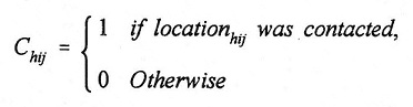 |
Chij was set to one for 2,764 locations and to zero for 181 locations where no contact was made.
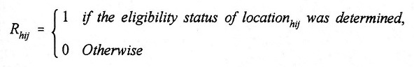 |
Because we assumed that locations that we were unable to contact were ineligible, Rhij was set to one for all selected locations except for the 296 locations that were contacted but not interviewed.
| TABLE 10. Final Disposition of the Facility Screening Sample1 | ||||||||
| Disposition | Expected Size7 | Total | ||||||
| 11-50 Beds | 51+ Beds | Unknown | ||||||
| # | Col % | # | Col % | # | Col % | # | Col % | |
| Responding Locations | ||||||||
| Eligibles | ||||||||
| 11 - 50 Beds2 | 363 | 43.5% | 192 | 14.6% | 28 | 3.5% | 583 | 19.8% |
| 51+ Beds2 | 44 | 5.3% | 590 | 44.8% | 34 | 4.3% | 668 | 22.7% |
| 407 | 48.7% | 782 | 59.4% | 62 | 7.8% | 1,251 | 42.5% | |
| Ineligibles | ||||||||
| Facilities | ||||||||
| 11 Beds3 | 84 | 10.1% | 104 | 7.9% | 101 | 12.7% | 289 | 9.8% |
| Ind. Living Only | 0 | 0.0% | 0 | 0.0% | 359 | 45.3% | 359 | 12.2% |
| Other Ineligible4 | 124 | 14.9% | 188 | 14.3% | 86 | 10.8% | 389 | 13.2% |
| Not a Facility5 | 56 | 6.7% | 43 | 3.3% | 72 | 9.1% | 171 | 5.8% |
| 264 | 31.7% | 335 | 25.4% | 618 | 77.9% | 1,217 | 41.3% | |
| Non-Responding Locations | ||||||||
| Contacted | ||||||||
| Refused | 79 | 9.5% | 125 | 9.5% | 20 | 2.5% | 224 | 7.6% |
| Not Interviewed6 | 25 | 3.0% | 40 | 3.0% | 7 | 0.9% | 72 | 2.4% |
| Unable to Contact8 | 60 | 7.2% | 35 | 2.7% | 86 | 10.8% | 181 | 6.2% |
| 164 | 19.6% | 200 | 15.2% | 113 | 14.2% | 477 | 16.2% | |
| TOTAL | 835 | 100% | 1,317 | 100% | 793 | 100% | 2,945 | 100% |
| ||||||||
Next, we used the indicators to compute the following non-response adjustment factor for each size stratum h:
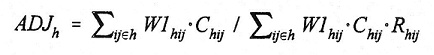 |
The adjustment factor is the ratio of the multiplicity-adjusted sampling weights among contacted locations divided by the corresponding weight sum for locations whose eligibility status was determined.
Finally, we calculated the non-response adjusted weight for each contacted location hij in size stratum h as:
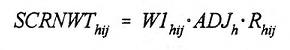 |
The sampling weights of the 181 non-contacted locations were not adjusted because they were assumed to be ineligible. Note that the non-response-adjusted weights of non-responding locations are zero. Also, the sum of the non-response adjusted weights in each size stratum h equals the sum of the multiplicity-adjusted weights for all selected locations in the stratum.
To estimate the total number of locations with one or more survey-eligible facilities in the national population, we first assigned the following indicator to each of the 2,649 locations with a known eligibility status:
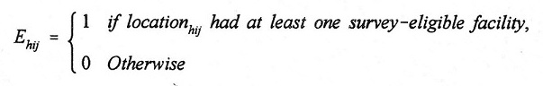 |
The eligibility indicator was set to one for 1,251 selected locations and to zero for 1,398 locations. The weighted sum of the eligibility indicator is 9,820 and provides an estimate of the total number of locations nationwide with one or more survey-eligible facilities. The 95 percent confidence interval of the estimate is +/- 1,137.
The estimated total number of survey-eligible ALFs in stratum h is:
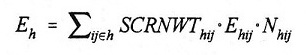 |
where
Nhij = the number of survey-eligible ALFs at location hij.
| TABLE 11. Estimated National Distribution of Eligible Facilities by Privacy and Service Levels | ||||
| Level of Service | Level of Privacy | Total | ||
| High | Low | Minimal | ||
| High | 1,265 + 2931 Tier #3 | 1,329 + 280 Tier #3 | 930 + 245Tier #1 | 3,524 + 574 |
| Low | 2,112 + 414Tier #3 | 3,081 + 568Tier #2 | 2,258 + 420 Tier #1 | 7,450 + 954 |
| Minimal | 222 + 88Tier #1 | 212 + 96Tier #1 | 64 + 47Tier #1 | 498 + 154 |
| Total | 3,598 + 617 | 4,622 + 706 | 3,252 + 510 | 11,471 + 1,272 |
| ||||
The sum of this estimator across all 1,251 eligible locations in the sample is 11,471 and provides an estimate of the total number of survey-eligible facilities in the target population. The 95 percent confidence interval is +/- 1,272. Because all facilities at each selected location were screened, the adjusted weight assigned to the facility is the same as the adjusted weight assigned to the location. Table 11 shows the distribution of the estimated number of eligible facilities by their levels of privacy and service.
Expected Statistical Power. For each combination of level of privacy and level of service, we calculated the expected pairwise percentage differences that can be detected by hypothesis tests or expected detectable differences among all eligible facilities that were identified in the facility screening. The expected detectable differences for each interaction and composite comparisons are shown in Table 12. The effective sample size is the number of eligible facilities in the comparison divided by its associated expected or average design effect.
| TABLE 12. Expected Detectable Differences1 for Comparing Percentage Estimates between Tier #1, #2, and #3 Facilities Identified during the Facility Screening2 | |||
| Design Effect | Effective Sample Size | Expected Detectable Difference | |
| Interactive Comparisons | |||
| High Privacy & High Service vs. High Privacy & Low Service | 1.31 | 393 | 12.6% |
| High Privacy & High Service vs. Low Privacy & High Service | 1.30 | 310 | 14.0% |
| High Privacy & High Service vs. Low Privacy & Low Service | 1.30 | 439 | 12.2% |
| High Privacy & High Service vs. Minimal Privacy & High Service | 1.30 | 258 | 15.8% |
| High Privacy & High Service vs. Minimal Privacy & Low Service | 1.29 | 363 | 13.0% |
| High Privacy & Low Service vs. Low Privacy & High Service | 1.31 | 377 | 13.0% |
| High Privacy & Low Service vs Low Privacy & Low Service | 1.31 | 506 | 11.0% |
| High Privacy & Low Service vs. Minimal Privacy & High Service | 1.32 | 325 | 15.0% |
| High Privacy & Low Service vs. Minimal Privacy & Low Service | 1.31 | 430 | 11.9% |
| Low Privacy & High Service vs. Low Privacy & Low Service | 1.30 | 423 | 12.6% |
| Low Privacy & High Service vs. Minimal Privacy & High Service | 1.30 | 243 | 16.1% |
| Low Privacy & High Service vs. Minimal Privacy & Low Service | 1.29 | 347 | 13.4% |
| Low Privacy & Low Service vs. Minimal Privacy & High Service | 1.30 | 372 | 14.6% |
| Low Privacy & Low Service vs. Minimal Privacy & Low Service | 1.30 | 476 | 11.5% |
| Minimal Privacy & High Service vs. Minimal Privacy & Low Service | 1.30 | 295 | 15.3% |
| Main Effects Comparisons (Assuming no interactions) | |||
| Tier #1 vs Tier #2 | 1.31 | 621 | 10.0% |
| Tier #1 vs Tier #3 | 1.31 | 885 | 8.5% |
| Tier #2 vs Tier #3 | 1.31 | 812 | 9.2% |
| High Privacy vs. Low Privacy | 1.31 | 856 | 8.5% |
| High Privacy vs. Minimal Privacy | 1.32 | 714 | 9.4% |
| Low Privacy vs. Minimal Privacy | 1.31 | 741 | 9.3% |
| High Service vs. Low Service | 1.32 | 1,099 | 7.8% |
| |||
3.2 Tier #2 and Tier #3 Facility Weights
Non-response Adjustments for Tier #2 and Tier #3 Facilities. During the administrator telephone recruitment, a number of facilities that had been considered eligible after the facility screening process were found to be ineligible. Some facilities had closed or merged with other facilities at the same location during the time lag from the screening to the telephone recruitment. Out of 241 Tier #2 facilities, 13 were found to be ineligible. For the Tier #3 facilities, 44 facilities were determined to be ineligible out of a total 482 facilities.
Since only one questionnaire was used for the Tier #2 facilities, a Tier #2 facility was classified as a respondent if the administrator responded to the Administrator Telephone Interview. From the 228 eligible facilities, there were 204 responding Tier #2 facilities.
Defining a respondent for a Tier #3 facility was much more complicated. Each facility could have Administrator In-person, Administrator Self-Administered and Walk-Through Observation Questionnaires, in addition to the Staff Member, Resident, Resident Proxy and Family Member questionnaires. Table 13 shows the distribution of the completed questionnaires for Tier #3 facilities. A responding facility was defined as one in which we received (at least) one questionnaire from at least one of the following four groups:
- Administrator In-Person Questionnaire
- Staff Member Questionnaire
- Resident, Resident Proxy or Family Member Questionnaires
This definition of response produced 300 Tier #3 facilities classified as respondents out of the 438 total facilities that were eligible.
We created weighting classes to adjust for possible differential participation rates across levels of privacy, service and size. For levels of privacy and service, we used the classifications of High and Low as shown in Table 11. For the size of the facility, we used the same 2 levels that were used in calculating the facility screening non-response adjustments (see section 3.1). Because the classification of facilities into Tier #2 and Tier #3 uses the levels of privacy and service as shown in Table 1, all of the Tier #2 facilities are included in the 2 size categories with low privacy and low service and the Tier #3 facilities are spread across the remaining 6 weighting classes pertaining to combinations of low and high levels of privacy and service and the 2 size categories.
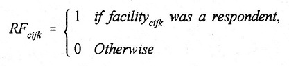
The following indicators were produced to classify all of the 723 Tier #2 and Tier #3 facilities, as indexed by facility k in location j in FSU i and classified in weighting class c:
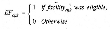 |
EFcijk was assigned a value of one for the 666 eligible facilities and to zero for the 57 ineligibles.
According to the above definitions of response, 504 facilities were given a value of one and the remaining 219 non-responding facilities were assigned a value of zero for RFcijk.
 |
| TABLE 13. Distribution of Questionnaires Obtained from Eligible Tier #3 Facilities1 | ||||||
| Administrator Supplement | Administrator In Person | Walk Through | Staff2 | Resident3 | Frequency | Percent |
| 133 | 30.4 | |||||
| X | 1 | 0.2 | ||||
| X | X | X | 3 | 0.7 | ||
| X | X | X | 1 | 0.2 | ||
| X | X | 1 | 0.2 | |||
| X | X | X | X | 44 | 10.1 | |
| X | 3 | 0.7 | ||||
| X | X | 1 | 0.2 | |||
| X | X | X | X | 1 | 0.2 | |
| X | X | 1 | 0.2 | |||
| X | X | X | 1 | 0.2 | ||
| X | X | X | 1 | 0.2 | ||
| X | X | X | X | 4 | 0.9 | |
| X | X | X | X | 3 | 0.7 | |
| X | X | X | X | X | 240 | 54.8 |
| 255 | 296 | 299 | 293 | 293 | 438 | |
| ||||||
The non-response adjustments for the Tier #2 and Tier #3 facilities were then calculated as follows for each weighting class c:
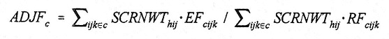 |
The final facility-level weight for the 504 responding facilities was calculated as:
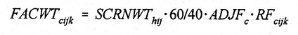 |
The term 60/40 reflects the weight adjustment for the subsample of 40 FSUs selected from the original 60 FSUs. Table 14 shows both the weighted and unweighted facility-level response rates for the Tier #2 and Tier #3 facilities.
Expected Statistical Power. We estimated the probability or power to detect pairwise percentage differences for outcomes related to Tier #2 and Tier #3 facilities by level of privacy and level of service. We based the power calculations on the expected (or average) design effects for each combination of privacy and service shown in Table 15. The effective sample size shown in the table is the number of respondents associated with the difference divided by the associated design effect.
| TABLE 14. Tier #2 and Tier #3 Facility-Level Response Rates | |||||||
| Weighting Classes | Eligible Facilities | Respondents | Response Rates | ||||
| Level of Privacy | Level of Service | Size1 | Unweighted | Weighted | |||
| Tier #3 | High | High | Medium | 73 | 51 | 69% | 72% |
| High | High | Large | 61 | 42 | 70% | 71% | |
| High | Low | Medium | 117 | 80 | 68% | 69% | |
| High | Low | Large | 80 | 51 | 64% | 65% | |
| Low | High | Medium | 46 | 31 | 67% | 69% | |
| Low | High | Large | 61 | 45 | 74% | 77% | |
| Subtotal: Tier #3 | 438 | 300 | 68% | 70% | |||
| Tier #2 | Low | Low | Medium | 121 | 109 | 91% | 90% |
| Low | Low | Large | 107 | 95 | 89% | 88% | |
| Subtotal: Tier #2 | 228 | 204 | 89% | 88% | |||
| Total | 666 | 504 | 76% | 77% | |||
| |||||||
| TABLE 15. Expected Detectable Differences1 for Comparing Percentage Estimates between Tier #2 and Tier #3 Facilities with Various Combinations of Privacy and Service | |||
| Design Effect | Effective Sample Size | Expected Detectable Difference | |
| Interactive Comparisons | |||
| High Privacy & High Service vs. High Privacy & Low Service | 1.34 | 167 | 19.2% |
| High Privacy & High Service vs. Low Privacy & High Service | 1.35 | 126 | 21.7% |
| High Privacy & High Service vs. Low Privacy & Low Service | 1.36 | 218 | 17.8% |
| High Privacy & Low Service vs. Low Privacy & High Service | 1.33 | 156 | 20.2% |
| High Privacy & Low Service vs. Low Privacy & Low Service | 1.35 | 248 | 15.9% |
| Low Privacy & High Service vs. Low Privacy & Low Service | 1.35 | 207 | 19.0% |
| Main Effects Comparisons (Assuming no interactions) | |||
| High Privacy vs. Low Privacy | 1.35 | 373 | 12.8% |
| High Service vs. Low Service | 1.35 | 373 | 13.5% |
| Tier #2 vs. Tier #3 | 1.35 | 373 | 13.0% |
| |||
3.3 Resident and Staff Member Weights
Non-response Adjustments for Residents and Staff Members. As in the classification of respondents for the Tier #2 and Tier #3 facilities, the definition for a staff member as being a respondent if we received the Staff Member Questionnaire was very straightforward, but the classification of a resident respondent involved a few possibilities. A resident was classified as a respondent if we received a Resident, Resident Proxy or a Family Member Questionnaire for the selected resident. From the 300 participating facilities, we received a total of 569 Staff Member Questionnaires out of the 615 staff members who were selected to be interviewed and classified 1,581 of the 1,802 selected residents as respondents.
The only indicators needed for the weight adjustments are to distinguish respondents from non-respondents:
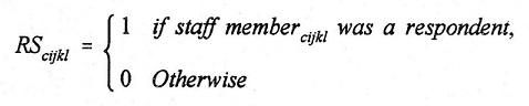 |
RScikjl was set to one for the 569 staff member respondents and set to zero for the other 46 non-respondents
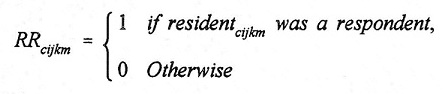 |
For the 1,581 resident respondents, RRcijkm was assigned a value of one and the remaining 221 non-responding residents were assigned a value of zero.
The non-response weight adjustments were calculated using the same weighting classes that were used in the Tier #2 and Tier #3 facility non-response adjustments:
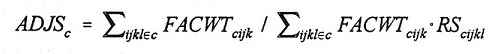 |
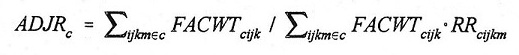 |
The final staff and resident weight adjustments were calculated from the final facility level weights as follows:
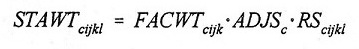 |
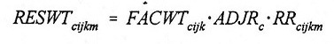 |
Table 16 and Table 17 show the weighted and unweighted response rates for the staff members and residents in the participating facilities. The response rates are calculated out of the total number of residents and staff members who were selected for the interviews in the 300 participating facilities.
| TABLE 16. Staff Member Response Rates in Participating Tier #3 Facilities | ||||||
| Weighting Classes | Total Staff Members | Respondents | Response Rates | |||
| Level of Privacy | Level of Service | Size1 | Unweighted | Weighted | ||
| High | High | Medium | 105 | 98 | 93% | 91% |
| High | High | Large | 85 | 77 | 91% | 95% |
| High | Low | Medium | 166 | 151 | 91% | 94% |
| High | Low | Large | 103 | 99 | 96% | 98% |
| Low | High | Medium | 66 | 60 | 91% | 91% |
| Low | High | Large | 90 | 84 | 93% | 98% |
| Total | 615 | 569 | 93% | 95% | ||
| ||||||
| TABLE 17. Resident Response Rates in Participating Tier #3 Facilities | ||||||
| Weighting Classes | Total Residents | Respondents | Response Rates | |||
| Level of Privacy | Level of Service | Size1 | Unweighted | Weighted | ||
| High | High | Medium | 306 | 281 | 92% | 93% |
| High | High | Large | 252 | 234 | 93% | 93% |
| High | Low | Medium | 482 | 416 | 86% | 92% |
| High | Low | Large | 306 | 268 | 88% | 91% |
| Low | High | Medium | 186 | 168 | 90% | 87% |
| Low | High | Large | 270 | 214 | 79% | 84% |
| Total | 1,802 | 1,581 | 88% | 90% | ||
| ||||||
As shown by the above response rate tables, the refusal rate of residents and staff members was very low for the 300 Tier #3 facilities that met the previously mentioned respondent criteria.
REFERENCES
Chong, E.K.P. and Zak, S.H. (1996). An Introduction to Optimization. John Wiley & Sons, New York.
Chromy, J.R. (1979). "Sequential Sample Selection Methods," Proceedings of the American Statistical Association, Section on Survey Research Methods, pp 401-406.
Fan, C.T., Muller, M.E, and Rezucha, I. (1962). "Development of Sampling Plans by Using Sequential (Item by Item) Selection Techniques and Digital Computers," Journal of the American Statistical Association, 57, 387-402.
Kish, L. (1965). Survey Sampling. John Wiley & Sons, New York.
Hawes, C., V. Mor, J. Wildfire, L. Lux, R. Green, V. Iannacchione, and C. Phillips (1995a). "Executive Summary: Analysis of the Effects of Regulation on the Quality of Care in Board and Care Homes." U.S. Department of Health and Human Services, Office of the Assistant Secretary for Planning and Evaluation, Washington, DC. [http://aspe.hhs.gov/daltcp/reports/care.htm]
Hawes, C., L. Lux, J. Wildfire, R. Green, L. Packer, V. Iannacchione, and C. Phillips (1995b). "Study of North Carolina Domiciliary Care Home Residents." Prepared for the North Carolina Department of Human Resources.
Mollica, R. and K. Snow (1996). State Assisted Living Policy: 1996. Portland, ME: National Academy for State Health Policy. [http://aspe.hhs.gov/daltcp/reports/96state.htm]
Thompson, S.K. (1992). Sampling. John Wiley & Sons, New York.
APPENDIX A: CLASSIFICATON OF FACILITIES WITH MISSING OR CONFLICTING DATA
In a number of instances, project staff classified facilities with missing or contradictory information into the facility categories used in the study. The general approach taken in these decisions attempted to assure that no facility would incorrectly be placed in a higher classification than was warranted.
Below we outline the situations in which missing or contradictory information had to be dealt with and the decision rules used in these instances. A single item on the instrument focused on occupancy of bedrooms by more than one person. The item concerning single occupancy was constructed from a series of items on the instrument. The service items were all separate items.
A total of only 65 facilities were classified based on the decisions noted below. The bulk of these facilities (42) were classified as a result of the decision rule in situation #1.
Situation #1
Do any of the resident bedrooms, including those in apartments, house more than 2 unrelated people? = Yes, and % accommodations that are single occupancy =100
Forty-two facilities were classified as minimal privacy because the response to the query about more than 2 unrelated persons sharing bedrooms was yes, which took priority over the response concerning single occupancy.
Situation #2
Do any of the resident bedrooms, including those in apartments, house more than 2 unrelated people? = No, and % accommodations that are single occupancy is missing
Six facilities were classified as minimal privacy because the information about single occupancy is missing, though the question about more than two people sharing a bedroom was answered no.
Situation #3
Do any of the resident bedrooms, including those in apartments, house more than 2 unrelated people? is missing, and % accommodations that are single occupancy is missing
Three facilities were classified as minimal privacy because both Q11UA and PERSNG are missing.
Situation #4
Do any of the resident bedrooms, including those in apartments, house more than 2 unrelated people?) is missing, and % accommodations that are single occupancy is less than 80
Two facilities were classified as low privacy because PERSNG was less than 80%, which took priority over the question about more than two people sharing a bedroom being missing.
Situation #5
Do any of the resident bedrooms, including those in apartments, house more than 2 unrelated people? = No, and % accommodations that are single occupancy is less than zero
Four facilities were classified as low privacy because PERSNG is less than zero, which in this instance takes precedent over the question about more than two people sharing a bedroom.
Situation #6 (services provided or arranged)
Two meals a day = Yes and Housekeeping = Yes and 24-hour staff oversight = Yes and Medication reminders =Yes and Central storage or assistance with medications = Yes and Assistance with bathing = Yes and Assistance with dressing =Yes
Seven facilities were classified as minimal service because there was missing data for the questions concerning whether they provide or arrange care by licensed nurses and whether they employ a full-time RN.
Situation #7 (services provided or arranged)
Two meals a day =Yes and Housekeeping = Yes and 24-hour staff oversight = Yes and Medication reminders = Yes and Central storage or assistance with medications = Yes and Assistance with bathing =Yes and Assistance with dressing = Yes andCare by licensed nurse = Provide and Do you have an RN on staff who works at least 40 hours per week? = Yes
One facility was classified as low service because the initial screening item concerning providing or arranging care by a licensed nurse was not equal to Yes.
NOTES
-
Minimal levels also included facilities with missing or conflicting information about services and/or privacy. See Appendix A for a more detailed discussion of facility classification in these circumstances.
-
A candidate ALF is a facility that proclaims itself as assisted living either by licensing status, association membership, classification in the Directory of Retirement Facilities, or by advertising in the Yellow Pages, and has eleven or more beds that serve the elderly. For coverage purposes, self-proclaimed ALFs with unknown capacities were also considered candidate ALFs.
-
Assisted Living Federation of America (ALFA), American Association of Homes and Services for the Aged (AAHSA), National Association of Residential Care Facilities (NARCF), and American Health Care Association (AHCA).
-
Explicit stratification ensures that a pre-specified number of sampling units of a certain type are selected. Within an explicit stratum, implicit stratification ensures proportional representation of factors believed to be related to study outcomes by systematic sampling from an ordered frame.
-
Because we intended to over-sample candidate ALFs with 51 or more beds, these facilities were assigned a larger weight than other candidate ALFs.
-
The cumulative design effect through the selection of the screening sample is expected to dominated by an unequal weighting effect of 1.11. Additional design effects were incurred when the sampling weights are adjusted for non-response and when the Tier #3 ALFs are sub-sampled for onsite data collection.
-
ALFs to be eligible for the survey were asked additional questions about the levels of service and privacy offered to their residents. We assumed that the incremental cost of asking these additional questions was minimal.
-
The effective sample size is the actual sample size divided by the design effect. Disproportionate sample allocations tend to have an effective sample size that is less than the actual sample size.
-
Nonlinear constrained optimization is used to find optimal solutions for problems that are nonlinear in nature and subject to a number of constraints. To minimize the unequal weighting effect (and hence maximize the effective sample size), we used quadratic extrapolation with central differencing for estimates of the partial derivatives of the objective and constraint functions. Details of the procedure may be found in Part IV of Chong & Zak, 1996.
OTHER REPORTS AVAILABLE
- A National Study of Assisted Living for the Frail Elderly: Discharged Residents Telephone Survey Data Collection and Sampling Report
- HTML http://aspe.hhs.gov/daltcp/reports/drtelesy.htm
- PDF http://aspe.hhs.gov/daltcp/reports/drtelesy.pdf
- A National Study of Assisted Living for the Frail Elderly: Final Sampling and Weighting Report
- HTML http://aspe.hhs.gov/daltcp/reports/sampweig.htm
- PDF http://aspe.hhs.gov/daltcp/reports/sampweig.pdf
- A National Study of Assisted Living for the Frail Elderly: Final Summary Report
- HTML http://aspe.hhs.gov/daltcp/reports/finales.htm
- PDF http://aspe.hhs.gov/daltcp/reports/finales.pdf
- A National Study of Assisted Living for the Frail Elderly: Report on In-Depth Interviews with Developers
- Executive Summary http://aspe.hhs.gov/daltcp/reports/indpthes.htm
- HTML http://aspe.hhs.gov/daltcp/reports/indepth.htm
- PDF http://aspe.hhs.gov/daltcp/reports/indepth.pdf
- A National Study of Assisted Living for the Frail Elderly: Results of a National Study of Facilities
- Executive Summary http://aspe.hhs.gov/daltcp/reports/facreses.htm
- HTML http://aspe.hhs.gov/daltcp/reports/facres.htm
- PDF http://aspe.hhs.gov/daltcp/reports/facres.pdf
- Assisted Living Policy and Regulation: State Survey
- HTML http://aspe.hhs.gov/daltcp/reports/stasvyes.htm
- PDF http://aspe.hhs.gov/daltcp/reports/stasvyes.pdf
- Differences Among Services and Policies in High Privacy or High Service Assisted Living Facilities
- HTML http://aspe.hhs.gov/daltcp/reports/alfdiff.htm
- PDF http://aspe.hhs.gov/daltcp/reports/alfdiff.pdf
- Family Members' Views: What is Quality in Assisted Living Facilities Providing Care to People with Dementia?
- HTML http://aspe.hhs.gov/daltcp/reports/fmviews.htm
- PDF http://aspe.hhs.gov/daltcp/reports/fmviews.pdf
- Guide to Assisted Living and State Policy
- HTML http://aspe.hhs.gov/daltcp/reports/alspguide.htm
- PDF http://aspe.hhs.gov/daltcp/reports/alspguide.pdf
- High Service or High Privacy Assisted Living Facilities, Their Residents and Staff: Results from a National Survey
- Executive Summary http://aspe.hhs.gov/daltcp/reports/hshpes.htm
- HTML http://aspe.hhs.gov/daltcp/reports/hshp.htm
- PDF http://aspe.hhs.gov/daltcp/reports/hshp.pdf
- National Study of Assisted Living for the Frail Elderly: Literature Review Update
- Abstract HTML http://aspe.hhs.gov/daltcp/reports/ablitrev.htm
- Abstract PDF http://aspe.hhs.gov/daltcp/reports/ablitrev.pdf
- HTML http://aspe.hhs.gov/daltcp/reports/litrev.htm
- PDF http://aspe.hhs.gov/daltcp/reports/litrev.pdf
- Residents Leaving Assisted Living: Descriptive and Analytic Results from a National Survey
- Executive Summary http://aspe.hhs.gov/daltcp/reports/alresdes.htm
- HTML http://aspe.hhs.gov/daltcp/reports/alresid.htm
- PDF http://aspe.hhs.gov/daltcp/reports/alresid.pdf
- State Assisted Living Policy: 1996
- Executive Summary http://aspe.hhs.gov/daltcp/reports/96states.htm
- HTML http://aspe.hhs.gov/daltcp/reports/96state.htm
- PDF http://aspe.hhs.gov/daltcp/reports/96state.pdf
- State Assisted Living Policy: 1998
- Executive Summary http://aspe.hhs.gov/daltcp/reports/98states.htm
- HTML http://aspe.hhs.gov/daltcp/reports/98state.htm
- PDF http://aspe.hhs.gov/daltcp/reports/98state.pdf
INSTRUMENTS AVAILABLE
- Facility Screening Questionnaire
- PDF http://aspe.hhs.gov/daltcp/instruments/FacScQ.pdf
To obtain a printed copy of this report, send the full report title and your mailing information to:
U.S. Department of Health and Human ServicesOffice of Disability, Aging and Long-Term Care PolicyRoom 424E, H.H. Humphrey Building200 Independence Avenue, S.W.Washington, D.C. 20201FAX: 202-401-7733Email: webmaster.DALTCP@hhs.gov
RETURN TO:
Office of Disability, Aging and Long-Term Care Policy (DALTCP) Home [http://aspe.hhs.gov/_/office_specific/daltcp.cfm]Assistant Secretary for Planning and Evaluation (ASPE) Home [http://aspe.hhs.gov]U.S. Department of Health and Human Services Home [http://www.hhs.gov]