
U.S. Department of Health and Human Services
Brookings/ICF Long Term Care Financing Model: Model Assumptions
David L. Kennell and Lisa Maria B. Alecxih, Lewin-ICF
Joshua M. Wiener and Raymond J. Hanley, Brookings Institution
February 1992
PDF Version (75 PDF pages)
This report was prepared under contract between the U.S. Department of Health and Human Services (HHS), Office of Disability, Aging and Long-Term Care Policy (DALTCP) and the Lewin Group. For additional information about the study, you may visit the DALTCP home page at http://aspe.hhs.gov/daltcp/home.htm or contact the ASPE Project Officer, John Drabek, at HHS/ASPE/DALTCP, Room 424E, H.H. Humphrey Building, 200 Independence Avenue, SW, Washington, DC 20201. His e-mail address is: John.Drabek@hhs.gov.
TABLE OF CONTENTS
A. The Models' Structure
B. Organization of the Documentation
II. KEY DEMOGRAPHIC AND RETIREMENT INCOME ASSUMPTIONS
A. PRISM Modeling System
B. Demographic Assumptions
C. Labor Force and Economic Assumptions
D. Pension Coverage Assumptions
E. Social Security and the Retirement Decision
F. Employer Pension Plan Assumptions
G. Individual Retirement Account Assumptions
H. Assets in Retirement
I. Supplemental Security Income Program Benefits
III. DISABILITY AND MORTALITY OF THE ELDERLY
A. Disability
B. Mortality
IV. LONG TERM CARE UTILIZATION
A. Nursing Home Utilization
A. Nursing Home Care Financing
B. Financing of Home Care Services
ATTACHMENTS (separate file)
Memo 1 (2/14/89): 1988 Social Security Trustee's and Bureau of the Census Population Projections
Memo 2 (6/6/89): SIPP Data on Support for Adults Living in Nursing Homes
Memo 3 (7/14/89): Status Report on Analysis of SIPP Data on Assets of the Elderly
Memo 4 (7/14/89): Profile of the SIPP Elderly Who Responded in 1984 but not 1985
Memo 5 (8/11/89): Update on Savings Rate of Elderly Families, 1984-1985
Memo 6 (10/18/89): Induced Demand
Memo 7 (10/19/89): Disability and Income
Memo 8 (1/9/90): Income and Asset Distribution of Elderly Families
Memo 9 (1/10/90): Additional Information on the Income and Asset Distribution of Elderly Families
Memo 10 (1/12/90): Additional Information on the Income and Asset Distribution of Elderly Families
Memo 11 (7/18/90): Life Insurance Values Held by the Elderly
Memo 12 (4/9/91): Table Specs for Distribution of Assets and Income
Memo 13 (4/25/91): Living Arrangement and Disability
Memo 14 (5/16/91): Medigap Analysis Results Using the 1984 SIPP/CES Match File and the 1989 CES
LIST OF FIGURES
FIGURE 1. Brookings/ICF Long Term Care Financing Model
FIGURE 2. Flowchart for Utilization of Long Term Care Services
FIGURE 3. Utilization of Formal Home Care by the Elderly
TABLE 1. Labor Force Participation Rates
TABLE 2. Unemployment Assumptions
TABLE 3. Consumer Price Index Assumptions Used In Forecasts
TABLE 4. Assumed Real Earnings Differentials
TABLE 5. Percent Distribution of Workers by Industry of Employment Assumed in PRISM for Selected Years
TABLE 6. Pension Coverage Assumptions
TABLE 7. Probabilities That Married Individuals Will Choose to Elect the Joint and Survivors Option, by Size of Pension Benefit
TABLE 8. Savings Plan Participation Assumptions
TABLE 9A. Proportion of DC LSDs That Are Rolled Over to an IRA, Pre-TRA
TABLE 9B. Proportion of DC LSDs That Are Rolled Over to an IRA, Post-TRA
TABLE 10. IRA Adoption Assumptions for Non-Covered Workers, by Age and Family Earnings Level
TABLE 11. IRA Adoption Probabilities for Covered Workers in 1982 by Family Income and Age of Worker
TABLE 12. Probabilities of Contributing to an IRA in a Given Year Once Selected to Adopt an IRA
TABLE 13. Distribution of Elderly Persons by Personal Income and Asset Levels, 1984
TABLE 14. Disability Prevalence Rates for the Noninstitutionalized
TABLE 15. Annual Disability Transition Probability Matrices for the Noninstitutionalized Elderly
TABLE 16. Disability Prevalence Rates for Noninstitutionalized Disability Insurance Recipients Simulated to Continue Being Disabled at Age 65
TABLE 17. Mortality Rates for the Noninstitutionalized Elderly in 1985
TABLE 18. Mortality Adjustments Used in the Model
TABLE 19. Annual Probability of Nursing Home Entry
TABLE 20. The Probability of Nursing Home Length of Stay by Age of Entry and Marital Status
TABLE 21. Number of Nursing Home Days Assigned by Length of Stay Category
TABLE 22. Nursing Home Disability Prevalence Rates
TABLE 23. Nursing Home Discharge Disability Prevalence Rate
TABLE 24. The Probability of Nursing Home Length of Stay by Age of Entry and Marital Status for Persons Using Services Due to Induced Demand
TABLE 25. Annual Probability of Starting to Use Formal Home Care Services for the Noninstitutionalized Chronically Disabled
TABLE 26. Annual Probability of Starting to Use Formal Home Care for Persons Who are Noninstitutionalized and Nondisabled at the Start of the Year
TABLE 27. Disability Level Prevalence Rates for Chronically Disabled Users of Paid Home Care
TABLE 28. Distribution of Home Care Length of Use for the Chronically Disabled
TABLE 29. Monthly Number of Formal Visits by Formal Home Care Disability Level
TABLE 30. Medicare Reimbursed Home Health Visits
TABLE 31. Percentage of Noninstitutionalized Non-Chronically Disabled Persons Receiving Medicare Home Health Visits
TABLE 32. Informal Home Care Prevalence Rates for the Chronically Disabled
TABLE 33. Average Daily Rates for Nursing Home Care by Source of Payment
TABLE 34. Medicare Part B Premium and Monthly Medigap Premiums
TABLE 35. Home Sale Patterns of Single Nursing Home Entrants
TABLE 36. Probability of Reduced Assets Upon Admission to a Nursing Home
TABLE 37. Likelihood of Receiving Medicare SNF Coverage and Length of Coverage
TABLE 38. Revised Medicaid Home Care Coverage Probabilitiesa for Persons with Assets Below SSI Level
TABLE 39. Out-of-Pocket and Other Payer Home Care Financing Assignment
TABLE 40. Average Prices Per Visit for Home Care by Source of Payment in 1988
OVERVIEW OF THE PROJECT
In September of 1988, the Office of the Assistant Secretary for Planning and Evaluation (ASPE) contracted with Lewin-ICF and the Brookings Institution to develop a public use version of the Brookings/ICF Long Term Care Financing Model. Using microsimulation techniques, the model projects the utilization and sources of financing for nursing home and home care services among the elderly to the year 2020.
Under this contract, many of the assumptions used in the model were revised to reflect data and findings that had recently become available. As the need for alternative policy simulations arose, the capabilities of the model were expanded. Examples of the types of simulations modeled include: the purchase of new private long term care insurance products; the use of pension funds to purchase long term care insurance; and publicly sponsored programs, such as the long term care benefits proposed by the Pepper Commission.
One of the products of this project is a public use version of the model code and accompanying documentation. The documentation includes:
Model Assumptions, which presents the assumptions used in developing the model.
Designing and Using Model Simulations, which presents assumptions used in modeling alternative proposals and using the results of the model.
A User's Guide to Specifying Simulations, which details how to specify simulations using the model's parameters.
A Programmer's/Operator's Manual, which shows the code structure and operation of the model.
PREFACE
This report is one of four related to the Brookings/ICF Long Term Care Financing Model. It outlines the assumptions used in developing the model. The three other documents discuss: 1) assumptions used in modeling alternative proposals and using the results of the model; 2) how to specify simulations using the model's parameters; and 3) the code structure and operation of the model.
This documentation was prepared by David L. Kennell and Lisa Maria B. Alecxih of Lewin-ICF in collaboration with Joshua M. Wiener and Raymond J. Hanley of the Brookings Institution. John Drabek, serving as the project officer, and Paul Gayer of the Office of the Assistant Secretary for Planning and Evaluation provided invaluable comments.
This report was developed as part of the documentation of a public use version of the Brookings/ICF Long Term Care Financing Model for the Office of the Assistant Secretary for Planning and Evaluation. Other reports in this series include:
- Designing and Using Model Simulations
- A User's Guide to Specifying Simulations
- A Programmer's/Operator's Manual
Copies of the reports may be obtained by writing to:Brenda Veazey, Department of Health and Human Services, Room 424E, Humphrey Building, 200 Independence Avenue, S.W., Washington, D.C. 20201
I. INTRODUCTION
A. The Models Structure
The Brookings/ICF Long Term Care Financing Model simulates the utilization and financing of long term care services -- both nursing home and home care -- for elderly individuals through 2020. Nursing home services include care provided by skilled nursing facilities (SNFs) and intermediate care facilities (ICFs). Home care services include home health, homemaker, personal care, and meal preparation services. The model simulates the number of individuals receiving these services and the costs of these services which are financed by various public and private sources. The overall objective of the model is to simulate the effects of various financing and organizational reform options on future public and private expenditures for nursing home and home care.
The two principal components of the model are the Pension and Retirement Income Simulation Model (PRISM) and the Long Term Care Financing Model. PRISM simulates future demographic characteristics, labor force participation, income and assets of the elderly. The Long Term Care Financing Model simulates disability, admission to and use of nursing home and home care, and methods of financing long term care services. The model uses national data and does not take into account regional, state or local variations.
The model begins with a nationally representative sample of the adult population with a record for each person's age, sex, income, and other characteristics. The model simulates changes for each individual's characteristics in the sample population from 1986 to 2020, including age, economic status, disability status, utilization of long term care, and the method of paying for such care.
The model uses a Monte Carlo simulation methodology. The model simulates changes in an individual's status by drawing a random number between zero and one and comparing it to the fixed probability of that event occurring for an individual with a given set of socio-demographic characteristics. For example, the annual probability of death for an 85 year old noninstitutionalized female is .03 (i.e., three out of every 100 women age 85 who are not in a nursing home are expected to die each year). If the random number drawn by the model is less than or equal to .03 for this 85 year old woman, then the individual is assumed to die in that year. If the number drawn lies between .03 and 1.0, then the individual is assumed to continue to live during that year. In order to reduce random variation due to the Monte Carlo procedure, the model is routinely run with two separate random number sets and the results are averaged.
The model can be used to simulate long term care financing assuming changes in private financing methods (such as increased purchase of private long term care insurance) or new public financing programs. These simulations are greatly affected by the choice of assumptions about the economy (such as the rate of growth of the overall economy and nursing home prices) and individual behavior (such as rates of nursing home utilization, insurance purchases, and induced demand). The model can be used to make estimates using alternative assumptions to show how sensitive the results are to the assumptions chosen.
The current version of the model is a major revision of the model that was developed jointly by Lewin-ICF and the Brookings Institution in 1986. The model was revised in 1988 and 1989 using data from a number of newly available data sources, including the 1982-84 National Long Term Care Survey, the 1985 National Nursing Home Survey, the 1984 Survey of Income and Program Participation (Wave 4), and Medicaid and Medicare program data provided by the Health Care Financing Administration (HCFA).
The six major components of the model are described below. A flowchart of these components is shown in Figure 1.
Population Data Base: Using data from the May 1979 Current Population Survey, the model uses information for a nationally representative sample of 28,000 adult individuals of all ages in 1979. This 1979 data base was chosen because it has been merged with social security earnings histories for each individual in the sample.
Income Simulator: The Pension and Retirement Income Simulation Model (PRISM) simulates labor force activity, marital status, income, and assets for each individual. The probabilities in this part of the model are based upon Census Bureau data on the likelihood of marriage, work, etc. for different demographic groups. The economic assumptions underlying the simulations are generally those used in Alternative 11-13 of the 1988 Social Security Trustee's Report. The model estimates retirement income from private sector defined benefit pension plans, public pension plans, social security, private sector defined contribution plans, Individual Retirement Accounts and Keoghs. The model also simulates the assets of elderly individuals including the value of home equity.
Disability of the Elderly: Using probabilities estimated primarily from the 1982-84 National Long Term Care Survey (NLTCS) and the 1985 National Nursing Home Survey (NNHS), this part of the model simulates the level of disability for persons age 65 and over. The model simulates the onset of disability, the level of disability, changes in disability, and recovery from disability.
Utilization of Long Term Care Services: This part of the model uses probabilities estimated from the 1982-84 NLTCS and the 1985 NNHS to simulate admission to and length of stay in a nursing home. For noninstitutionalized persons, the model also simulates the use and length of stay for paid home care services using probabilities derived primarily from the 1982-84 NLTCS and Medicare program data.
| FIGURE 1. Brookings/ICF Long Term Care Financing Model |
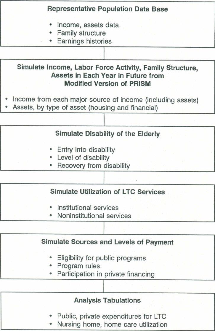 |
Sources and Levels of Payment: The fifth component of the model simulates the sources of payment and the level of expenditures for each individual receiving nursing home or home care services. The model incorporates Medicare eligibility and coverage provisions and uses a set of uniform assumptions about the Medicaid program, including provisions from the Medicare Catastrophic Coverage Act that were not repealed. State Medicaid program variations are not modeled.
Aggregate Expenditures and Utilization: The sixth part of the model accumulates Medicare, Medicaid, private expenditures, and utilization for each simulated individual for each year. The final output file from the model provides detailed information for individuals age 65 and older, for each year from 1986 to 2020, on individuals' age, sex, marital status, disability, sources and amounts of income, assets, and use of and payment sources for nursing home and home care services. This file is tabulated to show aggregate long term care expenditures for various demographic groups and sources of financing.
B. Organization of the Documentation
This document describes both the retirement income simulation and the long term care financing portions of the model. The retirement income simulations are described in more detail separately (see David L. Kennell and John F. Shells, "The ICF Pension and Retirement Income Simulation Model (PRISM) with the Brookings/ICF Long Term Care Financing Model," September 1986). Section II of the documentation describes the key demographic and retirement income assumptions in the model. Section III describes the probabilities used in the model to simulate disability and mortality for the elderly. Section IV describes the simulation of utilization of nursing home and home care services. Section V describes the financing of nursing home and home care services. Memos on data analyses related to the model are included as attachments.
II. KEY DEMOGRAPHIC AND RETIREMENT INCOME ASSUMPTIONS
The Pension and Retirement Income Simulation Model (PRISM) develops future estimates of retirement income.1 The model simulates retirement incomes for a sample of individuals age 25 and older in 1979 obtained from the ICF Pension/Social Security Data Base. The sources of income modeled in PRISM include: social security, employer pensions, Individual Retirement Accounts and Keogh accounts, employment earnings, asset income, and Supplemental Security Income (SSI) program benefits. PRISM simulates retirement income for this sample of the individuals based upon: (1) the characteristics of individuals in 1979; (2) their family and work histories prior to 1979; and (3) simulations of the future workforce experience of these individuals.
In order to simulate the future workforce experience and retirement incomes of these individuals, the model requires a large number of assumptions concerning the likelihood of future events for each individual, such as the likelihood an individual will continue to work, whether he or she will become divorced or married, and whether he or she will contribute to an IRA. These assumptions are divided into eight major areas:
- demographic
- labor force and economic;
- pension coverage;
- social security and the retirement decision;
- employer pension provisions;
- Individual Retirement Accounts;
- housing and financial assets; and
- Supplemental Security Income benefits.
The key assumptions used in each of these areas are summarized below. We start by briefly summarizing the PRISM modeling system.
A. PRISM Modeling System
The Pension and Retirement Income Simulation Model (PRISM) simulates the distribution of retirement income from both public and private resources for elderly families. PRISM models income from social security, private and public employee retirement plans, Individual Retirement Accounts (IRAs) and Keogh accounts, earnings, assets, and the Supplemental Security Income (SSI) program. It also estimates taxes paid in retirement.
The model simulates the distribution of retirement income among households of various socioeconomic groups for a representative sample of individuals age 25 and older in 1979 obtained from the ICF Pension/Social Security Database. These data are an exact match of the Special Pension Supplement to the May 1979 Current Population Survey (CPS) and Social Security Administration (SSA) earnings history data for 1951 through 1977.
For each individual in the population data base, PRISM uses probabilities estimated primarily from recent Census data to simulate each individual's earnings, periods of employment, and family structure between 1979 and the date of retirement. To ensure that PRISM simulations of labor force participation and earnings are consistent with the projected aggregate growth of the economy, we linked PRISM to the September 1987 labor force projections made by the Bureau of Labor Statistics.
Using the simulated work histories, the model calculates the social security benefits and IRA accumulations for each individual, as well as SSI benefits and earning from employment once the individual reaches retirement age, When individuals are simulated to enter a pension-covered job, the model assigns them to an actual pension plan sponsor selected from a representative sample of private and public retirement plan sponsors (the ICF Retirement Plan Provisions Data Base). When these individuals meet the plans' eligibility standards, PRISM then calculates their benefits using the plans' actual benefit provisions. This process of matching a representative sample of individuals to a representative sample of plan sponsors is a unique feature of PRISM. The model also estimates the amount of individuals' assets in retirement based upon the distribution of assets reported in the 1984 Panel of the Survey of Income and Program Participation (SIPP). Separate amounts are estimated for financial assets and home equity. Individuals are assumed to receive income from their nonhousing assets.
B. Demographic Assumptions
PRISM simulates mortality, disability, child bearing, and changes in marital status. During each simulation year, individuals are simulated to die, become disabled, recover from disability, bear children, and become married or divorced. The model uses a variety of assumptions to estimate these events, most of which are consistent with the Alternative II-B assumptions used in the 1988 report of the Trustees of the Old Age and Survivors Insurance and Disability Insurance Trust Funds (1988 Trustees' Report). The major assumptions are discussed below.
-
Mortality -- PRISM uses the Alternative II-B mortality assumptions used in the 1988 Trustees' Report. Mortality rates vary by age, sex, disability status, and years since becoming disabled. Mortality rates vary for each simulation year to reflect projected improvements in mortality made by the Social Security Actuaries. As discussed in a later section, mortality adjustments are made for persons 65 and over to reflect differences in mortality between institutionalized and noninstitutionalized, disabled and nondisabled persons.
-
Disability -- For persons under 65, PRISM uses the rates of disability used in the 1988 Trustees' Report. These rates vary by age and sex and are assumed to remain unchanged over time. Disability for persons age 65 and over is discussed in Section III.
-
Recovery from Disability -- For persons under 65, PRISM uses rates of disability recovery developed by the Social Security Actuaries for 1979-1980. These rates vary by age, sex, and years since becoming disabled. These are the most recent rates available and are assumed to remain unchanged over time. Recovery from disability for the elderly is discussed in Section III.
-
Child Bearing -- Fertility rates in the model are based upon an analysis of Census Bureau data on women who gave birth to children during the 1976-1980 period. These fertility rates vary by age, marital status, employment status, and number of children. In the model, these rates are constrained to match the Alternative II-B assumptions of fertility in the 1988 Trustees' Report.
-
Marital Status -- All probabilities concerning marriage and divorce are obtained from Monthly Vital Statistics data developed by the National Center for Health Statistics. The aggregate rates match the Alternative II-B projections in the 1988 Trustees' Report. Divorce rates vary by the age of husband and wife. Marriage rates vary by age, sex and marital status (i.e., never married, divorced, or widowed) of the individual. In the model, individuals selected to become married are joined with a member of the opposite sex based upon data on the distribution of newly married individuals by age and education of husband and wife reported in Vital Statistics data. The marriage and divorce rates are assumed to remain constant in the future.
C. Labor Force and Economic Assumptions
PRISM simulates each individual's employment history from 1979 (the date of the May 1979 CPS survey) through the date of retirement. During each simulation year, the model simulates wage rates, hours worked, job change and industry of employment. The simulations were constrained to match September 1987 Bureau of Labor Statistics (BLS) projections of employment and industry composition, and the Alternative II-B assumptions from the 1988 Trustees' Report of average wage rates in future years. The major assumptions are as follows:
-
Employment Levels Over Time -- PRISM was constrained to simulate aggregate levels of employment consistent with BLS forecasts of labor force participation rates for 1987-2000 (see Table 1).2 Labor force participation rates after 2000 are assumed to remain constant for each age/sex group. These forecasts include: 1) trends in employment for men and women of various age groups; 2) projections of economic growth; and 3) trends in the age of retirement. Unemployment rates from the 1988 Trustees' Report for the years 1986-2020 were used (see Table 2). Actual participation rates and unemployment rates are used for 1979 through 1987.
-
Employment by Socio-Economic Group -- Given the levels of labor force participation for different age/sex groups, the model simulates the number of hours each individual will work during each simulation year based upon an analysis of Bureau of the Census data on employment patterns during the 1976-80 period. For each individual, the decision to work and the number of hours worked in a year varies by age, sex, hours worked in each of the three previous years, marital status, presence of children at various ages, pension receipt status, and social security benefit receipt status.
-
Inflation -- Consumer prices are assumed to increase at the rate specified under the Alternative II-B assumptions in the 1988 Trustees' Report. These price change assumptions are shown in Table 3.
-
Interest Rates -- Assets in all defined contribution plans and individual retirement accounts (IRAs) were assumed to earn interest at an average annual rate of 7.0 percent.
-
Wage Growth -- Aggregate changes in wage levels are assumed to increase at the rate assumed in the Alternative II-B assumptions of the 1988 Trustees' Report (see Table 4). In general, average wages are assumed to grow by 1.3-1.6 percentage points in excess of the inflation rate in each year after 1990. Actual wage growth rates are used during the 1979-87 period. Given these aggregate rates, the hourly wage rates for each individual in the model are adjusted during each year based upon an analysis of Census Bureau data on patterns of wage growth. Rates of wage growth vary by age, sex, and whether or not the individual changed jobs during the year.
-
Job Change -- The probability that an individual will change jobs is based upon an ICF analysis of Census Bureau data concerning job change patterns during 1979. Job change is modeled as a function of the age, part-time/full-time status and job tenure of each worker. These probabilities are assumed to remain constant over time.
-
Maternity Job Terminations -- Women who have children often leave the labor force. In some instances, these women may re-enter the labor force and resume working for the same employers they had prior to having the child. In PRISM, we assume that a woman who has a child and leaves her job in the same year will become reemployed on the same job if: 1) the woman re-enters the labor force within five years of having the child; and 2) the woman became employed in the same industry she was in prior to having the child.
-
Industry Changes -- PRISM assigns individuals to an industry of employment when they change jobs or enter the labor force. The industry assigned to these individuals varies with age, full time/part time status, and industry of prior job. As shown in Table 5, the model assumes that over time, a higher proportion of workers work in the services industries and a lower proportion of workers work in the manufacturing industry. These industry composition estimates are based upon November 1987 BLS projections for the 1987-2000 period. After 2000, industry composition is assumed to remain constant.
| TABLE 1a. Labor Force Participation Rates | |||||||||||||||||
| 1984 | 1985 | 1986 | 1987 | 1988 | 1989 | 1990 | 1991 | 1992 | 1993 | 1994 | 1995 | 1996 | 1997 | 1998 | 1999 | 2000andAfter | |
| MEN | |||||||||||||||||
| 16-17 | 43.5 | 45.1 | 45.3 | 45.6 | 45.8 | 45.9 | 46.1 | 46.5 | 46.7 | 46.9 | 47.2 | 47.4 | 47.7 | 47.9 | 48.3 | 48.6 | 48.7 |
| 18-19 | 68.1 | 68.9 | 68.3 | 68.5 | 68.9 | 69.1 | 69.3 | 69.5 | 69.8 | 70.1 | 70.4 | 70.7 | 71.0 | 71.3 | 71.5 | 71.9 | 72.2 |
| 20-24 | 85.0 | 85.0 | 85.8 | 85.9 | 86.0 | 86.2 | 86.3 | 86.5 | 86.5 | 86.7 | 86.8 | 86.8 | 86.9 | 87.1 | 87.3 | 87.3 | 87.5 |
| 25-34 | 94.3 | 94.7 | 94.6 | 94.3 | 94.2 | 94.2 | 94.1 | 94.0 | 94.0 | 93.9 | 93.8 | 93.9 | 93.7 | 93.7 | 93.7 | 93.6 | 93.6 |
| 35-44 | 95.4 | 95.0 | 94.8 | 94.6 | 94.4 | 94.4 | 94.4 | 94.3 | 94.2 | 94.2 | 94.1 | 94.1 | 94.0 | 94.0 | 94.0 | 93.9 | 93.9 |
| 45-54 | 91.2 | 91.0 | 91.0 | 90.9 | 90.8 | 90.8 | 90.7 | 90.7 | 90.7 | 90.6 | 90.6 | 90.6 | 90.5 | 90.4 | 90.3 | 90.2 | 90.1 |
| 55-59 | 80.2 | 79.6 | 79.0 | 78.6 | 78.3 | 78.1 | 77.8 | 77.6 | 77.4 | 77.0 | 76.8 | 76.6 | 76.3 | 76.0 | 75.8 | 75.5 | 75.2 |
| 60-61 | 68.1 | 68.9 | 67.7 | 66.9 | 66.4 | 66.0 | 65.5 | 65.0 | 64.5 | 64.0 | 63.5 | 63.2 | 62.8 | 62.1 | 61.7 | 61.3 | 60.9 |
| 62-64 | 47.5 | 46.1 | 45.8 | 44.9 | 44.3 | 43.7 | 43.0 | 42.5 | 42.0 | 41.5 | 40.9 | 40.4 | 39.9 | 39.4 | 39.1 | 38.6 | 38.2 |
| 65-69 | 24.5 | 24.4 | 25.0 | 24.2 | 23.7 | 23.0 | 22.5 | 22.1 | 21.5 | 20.9 | 20.5 | 20.1 | 19.7 | 19.2 | 18.7 | 18.3 | 17.9 |
| 70-74 | 16.0 | 14.8 | 14.3 | 14.0 | 13.6 | 13.2 | 12.9 | 12.5 | 12.1 | 11.7 | 11.3 | 11.0 | 10.6 | 10.2 | 10.0 | 9.6 | 9.3 |
| 75+ | 7.5 | 7.0 | 7.1 | 7.0 | 6.8 | 6.5 | 6.3 | 6.1 | 5.8 | 5.7 | 5.4 | 5.2 | 5.1 | 4.9 | 4.7 | 4.5 | 4.3 |
| WOMEN | |||||||||||||||||
| 16-17 | 41.2 | 42.1 | 43.7 | 44.7 | 45.1 | 45.6 | 46.1 | 46.6 | 47.1 | 47.5 | 48.0 | 48.3 | 48.7 | 49.1 | 49.3 | 49.6 | 49.7 |
| 18-19 | 61.8 | 61.7 | 62.3 | 62.7 | 63.3 | 63.8 | 64.1 | 64.4 | 64.9 | 65.4 | 65.9 | 66.3 | 66.8 | 67.2 | 67.7 | 68.1 | 68.6 |
| 20-24 | 70.4 | 71.8 | 72.4 | 72.6 | 73.1 | 73.6 | 74.2 | 74.6 | 75.1 | 75.5 | 76.0 | 76.4 | 76.7 | 77.3 | 77.7 | 78.0 | 78.4 |
| 25-34 | 69.8 | 70.9 | 71.6 | 72.4 | 73.3 | 74.3 | 75.2 | 76.0 | 76.9 | 77.6 | 78.4 | 79.2 | 79.8 | 80.5 | 81.1 | 81.7 | 82.3 |
| 35-44 | 70.2 | 71.8 | 73.1 | 73.9 | 74.9 | 75.9 | 76.9 | 77.8 | 78.7 | 79.5 | 80.3 | 81.0 | 81.7 | 82.4 | 83.0 | 83.7 | 84.2 |
| 45-54 | 62.9 | 64.4 | 65.9 | 66.4 | 67.3 | 68.1 | 69.0 | 69.7 | 70.5 | 71.2 | 72.0 | 72.7 | 73.4 | 73.8 | 74.4 | 74.9 | 75.4 |
| 55-59 | 49.8 | 50.3 | 51.3 | 51.5 | 51.8 | 52.1 | 52.4 | 52.7 | 53.1 | 53.3 | 53.6 | 53.9 | 54.2 | 54.5 | 54.7 | 55.0 | 55.3 |
| 60-61 | 40.0 | 40.3 | 40.0 | 40.2 | 40.3 | 40.3 | 40.3 | 40.4 | 40.4 | 40.4 | 40.5 | 40.5 | 40.5 | 40.6 | 40.6 | 40.6 | 40.6 |
| 62-64 | 28.8 | 28.6 | 28.5 | 28.7 | 28.8 | 28.8 | 28.8 | 28.9 | 28.9 | 28.9 | 28.9 | 28.9 | 28.9 | 28.9 | 29.0 | 29.0 | 29.0 |
| 65-69 | 14.2 | 13.5 | 14.3 | 14.0 | 13.8 | 13.6 | 13.4 | 13.3 | 13.1 | 12.9 | 12.7 | 12.5 | 12.3 | 12.1 | 11.8 | 11.6 | 11.4 |
| 70-74 | 7.3 | 7.6 | 6.9 | 7.1 | 7.1 | 7.0 | 7.0 | 6.9 | 6.9 | 6.8 | 6.7 | 6.7 | 6.7 | 6.6 | 6.6 | 6.5 | 6.5 |
| 75+ | 2.5 | 2.2 | 2.4 | 2.4 | 2.4 | 2.3 | 2.2 | 2.1 | 2.1 | 2.0 | 1.9 | 1.9 | 1.8 | 1.7 | 1.7 | 1.6 | 1.5 |
SOURCE: Howard N. Fullerton, Jr., "Labor Force Projections 1986-2000," Bureau of Labor Statistics' Monthly Labor Review, September 1987. | |||||||||||||||||
| TABLE 2. Unemployment Assumptions | |
| Year | Average AnnualUnemployment Rate |
| 1979 | 5.8% |
| 1980 | 7.1 |
| 1981 | 7.6 |
| 1982 | 9.7 |
| 1983 | 9.6 |
| 1984 | 7.5 |
| 1985 | 7.2 |
| 1986 | 7.0 |
| 1987 | 6.2 |
| 1988 | 6.0 |
| 1989 | 6.2 |
| 1990 | 6.1 |
| 1991 | 6.0 |
| 1992 | 5.9 |
| 1993 | 5.8 |
| 1994 | 5.8 |
| 1995 | 5.8 |
| 1996 | 5.8 |
| 1997-1999 | 5.7 |
| 2000 and later | 6.0 |
| SOURCE: Alternative II-B assumptions from the 1988 Annual Report of the Board of Trustees of the Federal Old Age and Survivors Insurance and Disability Insurance Trust Funds, April 1988. | |
| TABLE 3. Consumer Price Index Assumptions Used In Forecasts | |
| Year | Annual Change inConsumer Price Index |
| 1979 | 11.4 |
| 1980 | 13.5 |
| 1981 | 10.3 |
| 1982 | 6.0 |
| 1983 | 3.0 |
| 1984 | 3.4 |
| 1985 | 3.5 |
| 1986 | 1.6 |
| 1987 | 3.6 |
| 1988 | 3.9 |
| 1989 | 4.5 |
| 1990 | 4.3 |
| 1991 | 4.2 |
| 1992 | 4.0 |
| 1993 | 4.0 |
| 1994 and later | 4.0 |
| SOURCE: 1988 Annual Report of the Board of Trustees of the Federal Old-Age and Survivors Insurance and Disability Insurance Trust Funds, Washington, D.C.: Social Security Administration, April 1988. | |
| TABLE 4. Assumed Real Earnings Differentials | |
| Year | Real EarningsDifferentiala |
| 1979 | -2.2% |
| 1980 | -4.4 |
| 1981 | -1.0 |
| 1982 | 0.6 |
| 1983 | 1.8 |
| 1984 | 2.3 |
| 1985 | 0.7 |
| 1986 | 2.8 |
| 1987 | -0.6 |
| 1988 | 0.9 |
| 1989 | 1.1 |
| 1990 | 1.1 |
| 1991 | 1.3 |
| 1992 | 1.7 |
| 1993 | 1.6 |
| 1994 | 1.6 |
| 1995 | 1.5 |
| 1996 | 1.5 |
| 1997 | 1.5 |
| 1998 | 1.4 |
| 1999 | 1.4 |
| 2000 and later | 1.4 |
SOURCE: Alternative II-B assumptions from the 1988 Annual Report of the Board of Trustees of the Federal Old Age and Survivors Insurance and Disability Insurance Trust Funds, April 1988. | |
| TABLE 5. Percent Distribution of Workers by Industry of Employment Assumed in PRISM for Selected Years | |||||
| Industry | 1980 | 1982 | 1984 | 1990 | 2000 andAfter |
| Mining | 0.59% | 0.95% | 1.30% | 0.88% | 0.78% |
| Construction | 4.53 | 4.20 | 4.44 | 4.81 | 4.62 |
| Manufacturing | 20.78 | 19.08 | 18.73 | 16.32 | 14.09 |
| Transportation | 5.02 | 5.03 | 5.32 | 4.96 | 4.74 |
| Trade | 18.71 | 19.24 | 19.26 | 19.86 | 20.58 |
| Finance | 5.09 | 5.32 | 5.38 | 6.09 | 6.06 |
| Service | 17.55 | 18.50 | 18.50 | 20.34 | 23.08 |
| State & Local | 12.96 | 12.96 | 12.61 | 12.29 | 11.73 |
| Federal | 3.28 | 3.28 | 3.26 | 3.07 | 2.79 |
| Self Employed | 9.55 | 9.85 | 9.63 | 10.06 | 10.45 |
| Agriculture | 1.64 | 1.65 | 1.55 | 1.29 | 1.07 |
| Total | 100.00% | 100.00% | 100.00% | 100.00% | 100.00% |
| SOURCE: Lewin-ICF estimates based upon George T. Silverstri and John M. Lukasiewicz, "A Look at Occupational Employment Trends to the Year 2000," Bureau of Labor Statistics' Monthly Labor Review, September 1987. | |||||
D. Pension Coverage Assumptions
For each job individuals have during the simulation, PRISM determines whether they are covered by a retirement plan and assigns covered workers to actual pension plan sponsors in the ICF Retirement Plan Provisions Data Base. Coverage rates were assumed to remain constant through time. The key assumptions are presented below.
-
Pension Coverage -- As workers change jobs or enter the labor force during the simulation, retirement plan coverage is simulated using coverage rates reported for job changers and labor force entrants in the May 1979 CPS. The model is further constrained to replicate coverage rates reported in the May 1983 EBRI/HHS CPS pension supplement. These coverage rates vary by the individual's industry of employment, full time/part time worker status, age, and real wage rate. Plan coverage on an industry basis is assumed not to change between 1983 and 1988 when the new nondiscrimination rules introduced in the 1986 Tax Reform Act became effective. The coverage rates assumed for 1979, 1983, and 1989 are presented in Table 6.
-
Impact of 1986 Tax Reform Act on Pension Coverage -- Internal Revenue Service's (IRS) pension plan nondiscrimination rules that became effective in 1989 stipulate that, in general, no more than 30 percent of a plan sponsor's employees could be excluded. Previously, employers could legally exclude up to 44 percent of their employees from the plan.3 The impact of this provision is modeled by estimating the number of persons in each industry who were not participating in a pension plan even though: (1) their employers sponsor a pension plan; and (2) they appear to meet the most restrictive age and service criteria allowed under ERISA (i.e., age 25 with at least 1,000 hours worked over a period of one year). In the model, the coverage rates for each industry are increased starting in 1989 so that no more than 30 percent of these individuals are not participating in their employer's plan (see Table 6).
-
Plan Assignment -- Individuals are assigned to plan sponsors in the ICF Retirement Plan Provisions Data Base in proportion to the number of individuals actually covered by that plan sponsor. PRISM assigns individuals to plans of similar industry, firm size, social security coverage status, union coverage status, multi/single employer plan status, and hourly/salary worker status. In addition, individuals are assigned only to plans which are consistent with the characteristics of the plan the individual reported he was covered by in the May 1979 CPS. To do this, the model takes into account the individual's reported participation and vesting status as well as plan contribution requirements and participation in a supplemental plan.
| TABLE 6. Pension Coverage Assumptions | |||
| Industry | Pension Coverage Rate | ||
| 1979 | 1983 | 1989 | |
| Federal Government | .93 | .93 | .93 |
| State & Local Government | .88 | .83 | .83 |
| Mining | .82 | .75 | .79 |
| Manufacturing | .76 | .70 | .73 |
| Transportation | .75 | .75 | .77 |
| Finance | .67 | .67 | .75 |
| Construction | .43 | .41 | .43 |
| Trade | .43 | .46 | .51 |
| Services | .43 | .47 | .52 |
| Agriculture | .19 | .22 | .22 |
| Self Employed | .14 | .14 | .14 |
| SOURCE: Coverage rates for 1979 were derived from an ICF analysis of the May 1979 Current Population Survey. Coverage rates for 1983 are based on an ICF analysis of the May 1983 EBRI/HHS CPS Pension Supplement. Coverage rates for 1989 were estimated by ICF by adjusting the 1983 coverage rates to reflect the potential impact of the nondiscrimination rules in the Tax Reform Act of 1986. | |||
E. Social Security and the Retirement Decision
The model simulates the acceptance of early, normal and late retirement benefits from both pension plans and social security. Current social security legislation provisions (including the 1983 amendments which increased the age at which unreduced benefits will be available) were assumed to be in place throughout the simulation. The important assumptions in the retirement decision are summarized below.
-
Social Security Benefit Acceptance -- PRISM simulates the age at which individuals start to receive social security benefits. These benefit acceptance rates vary by the age and sex of the individual. The rates were derived from social security benefit receipt data by age and sex during 1980. PRISM also assumes that eligible individuals age 62 or over will automatically accept benefits if they are disabled or unemployed or receiving an employer pension. These assumptions lead to an increase in social security early retirement because the number of individuals receiving pensions will increase over time in the simulations.
-
Social Security Survivors Benefits -- Individuals are simulated to accept social security survivors benefits in the first year they are eligible.
-
Employer Pension Benefit Acceptance -- PRISM determines when an individual is eligible to accept employer pension benefits and then simulates the decision to accept the benefit. Benefit acceptance rates were developed by ICF based upon an analysis of Census Bureau data on pension benefit recipients.
-
Impact of Eliminating Age 70 Mandatory Retirement -- Prior to 1987, employers could legally require workers to retire when they reached age 70. Legislation passed in 1986 made such regulations illegal for most employers. All plans in the ICF Retirement Plan Data Base were modified to eliminate mandatory retirement beginning in 1987. The BLS labor force participation projections take into account the expected impact of the elimination of mandatory retirement.
-
Acceptance of Deferred Vested Benefits -- Individuals who are vested and leave their job prior to their eligibility for early or normal retirement receive a deferred vested benefit. These benefits are assumed to go into pay status when the individual reaches the plan's normal retirement age.
F. Employer Pension Plan Assumptions
PRISM simulates the size of the benefit individuals will receive from each pension plan in which they earn a benefit during the simulation. PRISM uses the actual provisions of the plan to which the individual was assigned to determine each individual's eligibility and benefit amount. In general, pension plan provisions are assumed to remain unchanged over time except in instances where plan rules must be changed to be in compliance with the Retirement Equity Act of 1984 (REA) and the Tax Reform Act of 1986. The following assumptions are used:
-
Benefit Formulas -- The benefit formulas in defined benefit plans are indexed to changes in wages for flat and unit benefit formulas. Defined contribution plan salary bend points are also indexed to wage growth. Final pay defined benefit and all other parts of defined contribution plan formulas are held constant. No changes in participation, vesting or other plan provisions are assumed except where required by REA or the Tax Reform Act of 1986.
-
Impact of REA on Participation Rules -- REA mandated that starting in 1985, the minimum age requirement for participation would be reduced from 25 to 21 and that service between the age of 19 and 22 would be considered for determining vesting. Starting in 1985, the provisions of any private plans which were not already in compliance with these provisions are modified.
-
Impact of the Tax Reform Act of 1986 on Vesting -- The Tax Reform Act required private sector single-employer plans to vest benefits at least as rapidly as under the following two schedules: (1) full vesting upon completion of five years of service, or (2) 20 percent vesting after the completion of three years of service and 20 percent more for each subsequent year.4 Starting in 1989, the provisions of any private single employer plans which were not already in compliance with these provisions are modified.
-
Limits on Social Security Integration -- Private sector plans which integrate benefits with social security are required to limit their integration formulas. Although previous IRS regulations placed restrictions on how plans may integrate benefits, some low-wage workers had their pension benefits severely reduced or completely eliminated through integration. The Tax Reform Act retained and simplified IRS regulations on integration. In addition, the Act establishes additional restrictions on integration that apply separately to three types of integrated plans:
-
For defined benefit excess/step-rate (plans which calculate pension benefits at different rates on earnings above and below specified levels), the rate at which benefits are provided for pay up to the integration level of a plan (the compensation amount below which pension benefits are reduced) may not be less than 50 percent of the rate at which benefits are provided in excess of that level. In addition, the integration level may not be more than the social security wage and benefit base.
-
For defined benefit offset plans (plans where pension benefits are reduced by a stated percentage of the person's social security benefit), the offset may not reduce a participant's benefits by more than 50 percent.
-
For defined contribution plans (plans where the employer contributes a specified amount but does not guarantee a specified benefit), the provisions are similar except that they apply to the rate of employer contributions. In addition, for defined contribution plans, the rate for pay in excess of the integration level may not exceed the rate for up to that level by more than the OASDI tax rate.
-
-
Cost of Living Adjustments for Pensions -- The model assumes that benefits for private plan beneficiaries from defined benefit plans will be indexed at half of the rate of inflation up to a maximum of two percent per year. All early and normal retirement benefits from the Civil Service Retirement Plan are assumed to increase at the annual rates of inflation shown in Table 3. State and local government benefits are assumed to increase at the rate of inflation up to a maximum of four percent each year. These assumptions are based upon a prior ICF study which analyzed cost of living adjustments over a ten year period for a representative sample of pension plans. None of these plans are assumed to index deferred vested benefits.
-
Post-Retirement Survivors Benefit Option -- Table 7 presents the assumptions used to determine which married individuals choose to elect the post-retirement joint and survivors option. Because REA mandated that starting in 1985 spousal consent is required to waive survivors benefit coverage, the model assumes that the rate of joint and survivor election will increase after the act is implemented (see Table 7). Individuals who accept the post-retirement survivors option are assumed to receive a 50 percent joint and survivor's annuity. This annuity provides a surviving spouse with a benefit equal to half of that received by the deceased individual while living.
-
Pre-retirement Survivors Option -- Many plans automatically provide individuals with pre-retirement survivor's coverage. In these plans, all individuals are assumed to "elect" the pre-retirement survivors option. In the other defined benefit plans, the model assumes 60 percent of married individuals will elect the pre-retirement survivors option. Because REA mandated spousal consent for waiver of the survivors coverage, the model assumes that 85 percent of all married individuals elect this option after REA is implemented.
-
Vested Beneficial Survivors Benefits -- As mandated by REA, pre- retirement survivors coverage was extended to spouses of individuals who receive vested benefits. Thus, the model simulates survivors benefits for spouses of vested beneficiaries who die between the time they leave the job and the date the benefits would have gone into pay status. In all instances the survivors benefit is assumed to be a 50 percent joint and survivors annuity.
-
Maternity -- Under REA, workers who leave a pension plan may return to the job and retain their prior years of service for participation and vesting status provided the break in service was less than or equal to the greater of: (1) five years; or (2) the number of years of service prior to the break. Although both men and women may benefit from this provision, it was intended to assist women who leave their job for maternity. Because reemployment by the same employer is modeled in maternity cases only, this rule is applied only to women in the model who have children. In addition, due to further REA liberalizations in crediting service for maternity cases, working women who have a child are assumed to receive one year of credited service for the year the child is born, regardless of the number of hours they worked.
-
Participation in Savings, Thrift and 401(K) Plans -- Table 8 summarizes the assumptions on participation in supplemental thrift, savings and 401(K) plans for those individuals who are eligible to participate in them. The participation rates are a function of a worker's wage level and the employer matching rate.
-
Employee Contributions -- In plans which require employee contributions as a condition for plan participation, the model assumes individuals contribute the amount required to obtain the maximum employer contribution.
-
Lump Sum Payments -- In the current version of PRISM, individuals who are vested in a defined contribution plan and change jobs are selected to roll their lump sum payment into an IRA on the basis of lump sum rollover data obtained from an analysis of the May 1983 EBRI/HHS CPS Pension Supplement.5 The likelihood of a rollover varies by age, marital status, benefit level, and income. Among individuals age 55 or older, all lump sums over $1,750 are rolled over into an IRA and saved for retirement.
-
Impact of Tax Reform Act on Roll-Overs -- The Tax Reform Act eliminated 10 year averaging, thus increasing individuals' incentives to roll-over into an IRA lump sum distributions received from a pension plan. Individuals age 59½ or older are permitted to make a one-time election to use 5-year forward averaging for a lump sum distribution which is not rolled-over into an IRA. Also, individuals attaining age 50 prior to January 1, 1986, may also make a one time election to use 5 year averaging for a lump sum distribution. The proportion of individuals who roll-over lump-sum distributions and save these assets for retirements was increased by 20 percent to model the impact of these provisions. These assumptions are shown in Table 9A and Table 9B.
-
Lump Sum Payments at Retirement Income -- Individuals are assumed to draw upon their defined contribution lump sum payments (those which were not cashed out) in the form of an annuity. This annuity is assumed to start at the earlier of: (1) the age they accepted social security benefits or (2) the year they first started receiving a defined benefit pension, but not earlier than age 55.
| TABLE 7. Probabilities That Married Individuals Will Choose to Elect the Joint and Survivors Option, by Size of Pension Benefit | ||
| Pension Benfit Size(in 1980 dollars) | Probability of Choosing the Post-RetirementJoint and Survivor's Option | |
| Before REA | After REA | |
| Less than $3,000 | 25% | 75% |
| $3,000 or over | 65% | 80% |
| SOURCE: Lewin-ICF assumptions. | ||
| TABLE 8. Savings Plan Participation Assumptions | |||
| Hourly Wage Levela | Employer Match Rateb | ||
| Low | Medium | High | |
| Less than $4 | 20% | 25% | 30% |
| $4-$7 | 40% | 50% | 60% |
| More than $7 | 60% | 75% | 90% |
SOURCE: Lewin-ICF assumptions. | |||
| TABLE 9A. Proportion of DC LSDs That Are Rolled Over to an IRA, Pre-TRA | ||||||||||
| Earnings(1983 $s) | Under Age 30 | Age 30-34 | Age 45-54 | Age 55-61 | Age 62 or more | |||||
| $3,500 | $3,500+ | $3,500 | $3,500+ | $3,500 | $3,500+ | $3,500 | $3,500+ | $3,500 | $3,500+ | |
| NOT COLLEGE GRADUATE | ||||||||||
| $20,000 | 0.019 | 0.000 | 0.013 | 0.050 | 0.028 | 0.143 | 0.000 | 1.000 | 1.000 | 1.000 |
| $20,000+ | 0.024 | 0.000 | 0.041 | 0.091 | 0.105 | 0.211 | 0.000 | 1.000 | 1.000 | 1.000 |
| COLLEGE GRADUATE | ||||||||||
| $20,000 | 0.037 | 0.000 | 0.015 | 0.061 | 0.075 | 0.364 | 0.000 | 1.000 | 1.000 | 1.000 |
| $20,000+ | 0.040 | 0.154 | 0.051 | 0.178 | 0.120 | 0.450 | 0.000 | 1.000 | 1.000 | 1.000 |
| TABLE 9B. Proportion of DC LSDs That Are Rolled Over to an IRA, Post-TRA | ||||||||||
| Earnings(1983 $s) | Under Age 30 | Age 30-34 | Age 45-54 | Age 55-61 | Age 62 or more | |||||
| $3,500 | $3,500+ | $3,500 | $3,500+ | $3,500 | $3,500+ | $3,500 | $3,500+ | $3,500 | $3,500+ | |
| NOT COLLEGE GRADUATE | ||||||||||
| $20,000 | 0.023 | 0.000 | 0.016 | 0.060 | 0.034 | 0.172 | 0.000 | 1.000 | 1.000 | 1.000 |
| $20,000+ | 0.029 | 0.000 | 0.049 | 0.109 | 0.126 | 0.253 | 0.000 | 1.000 | 1.000 | 1.000 |
| COLLEGE GRADUATE | ||||||||||
| $20,000 | 0.044 | 0.000 | 0.018 | 0.073 | 0.090 | 0.437 | 0.000 | 1.000 | 1.000 | 1.000 |
| $20,000+ | 0.048 | 0.185 | 0.061 | 0.214 | 0.144 | 0.054 | 0.000 | 1.000 | 1.000 | 1.000 |
G. Individual Retirement Account Assumptions
PRISM models the accumulation of IRA savings. The assumptions used in this analysis are derived primarily from IRA participation data provided in the May 1983 EBRI/HHS CPS pension supplement. ICF recalibrated the assumptions used in these simulations so that PRISM assumptions are consistent with the 1983 estimates of: (1) the number of individuals participating in IRAs; and (2) the amount of IRA assets accumulated. The key assumptions in our IRA simulations are summarized below. In addition, we modified the IRA subroutine of PRISM to reflect the impact of the 1986 Tax Reform Act on IRA savings.
-
IRA Adoption for Non-Covered Workers -- Table 10 summarizes the assumptions used in modeling the adoption of IRAs by non-pension covered workers. These estimates do not include workers assumed to roll over vested benefits into IRA arrangements. ICF estimated these adoption rates using May 1983 EBRI/HHS CPS pension supplement data on non-covered individuals establishing an IRA during 1982.
-
IRAs for Covered Workers -- A separate set of IRA adoption probabilities were developed for individuals covered by a pension plan which apply only to 1982 (shown in Table 11). These probabilities were estimated using the May 1983 EBRI/HHS CPS pension supplement data on covered workers who established an IRA in 1982. In years after 1982, the IRA adoption rates for covered workers are assumed to be the same as for non-covered individuals (see Table 9), except as described below.
-
IRA Contributions -- Once an individual is selected to adopt an IRA, PRISM simulates his or her decision to contribute to the account for each year after the IRA is established. The model assumes that individuals contribute only if they are employed during the year. All individuals are assumed to contribute in the year the IRA is established. In succeeding years, individuals are randomly selected to contribute to their account based upon the probabilities presented in Table 12. These probabilities were estimated using May 1983 EBRI/HHS CPS pension supplement data on the number of individuals with IRA accounts who are currently contributing.
-
IRA Contribution Amount -- The amount that individuals are assumed to contribute to their IRA in a given year varies with family income, age, sex, and marital status. If an individual is selected to contribute to an IRA the model randomly selects the amount to be contributed based upon the distribution of IRA contributions reported in the May 1983 EBRI/HHS CPS pension supplement data for individuals in similar age, sex, income and marital status groups. The amounts of these contributions are indexed to real wage changes after 1983. The annual contribution is constrained not to exceed the maximum contribution allowed under the law. After 1986, the maximum contribution amounts specified in the law are indexed at 80 percent of the CPI over time (actual contribution limits are used for each year through 1986). Individuals who reported they had an IRA in 1979 were assumed to have an initial balance of $3,000 (in 1982 dollars) in their account.
-
Impact of Tax Reform Act of 1986 -- The Tax Reform Act modified the maximum tax deductible amount of contributions to IRAs for active participants in qualified pension, profit-sharing, stock-bonus, tax sheltered annuity or government plans. Beginning in 1987, the full contribution amount up to the amount deductible under prior tax law (typically $2,000) is deductible for individuals with Adjusted Gross Income under $25,000 ($40,000 for joint filers, $0 for married filing separately). The deductibility is phased out over the next $10,000 of AGI for the active participants. Anyone may make a non-deductible contribution to the extent that deductible IRA contributions are not allowed. The IRA deduction for all others is retained in its current form. Beginning in 1987, PRISM assumes that annual contributions to IRAs for pension plan participants are limited to the maximum deductible amount allowed for taxpayers at their income level (i.e., individuals will only contribute if the contribution is tax deductible).
| TABLE 10. IRA Adoption Assumptions for Non-Covered Workers, by Age and Family Earnings Level | ||||||
| Family Earnings Level | Age | |||||
| 25-34 | 35-39 | 40-44 | 45-54 | 55-59 | 60-65 | |
| Less than $15,000 | 0.24% | 0.24% | 0.48% | 0.48% | 0.72% | 0.96% |
| $15,000-24,999 | 0.96 | 0.96 | 1.20 | 1.44 | 1.68 | 2.16 |
| $25,000-29,999 | 1.20 | 1.32 | 1.44 | 2.40 | 2.40 | 3.60 |
| $30,000-34,999 | 1.80 | 2.40 | 3.60 | 4.20 | 4.80 | 6.00 |
| $35,000-49,999 | 3.60 | 3.60 | 4.20 | 4.80 | 6.00 | 8.40 |
| $50,000 or More | 6.00 | 6.00 | 6.00 | 6.00 | 12.00 | 12.00 |
| SOURCE: Lewin-ICF estimates, based in part upon the May 1983 EBRI/HHS CPS pension supplement data. | ||||||
| TABLE 11. IRA Adoption Probabilities for Covered Workers in 1982 by Family Income and Age of Worker | ||||||
| Family Earnings Level | Age | |||||
| 25-34 | 35-39 | 40-44 | 45-54 | 55-59 | 60-65 | |
| Less than $15,000 | 4.0% | 7.0% | 4.0% | 9.0% | 13.0% | 20.0% |
| $15,000-24,999 | 8.0 | 8.0 | 9.0 | 17.0 | 27.0 | 19.0 |
| $25,000-29,999 | 9.0 | 14.0 | 16.0 | 23.0 | 30.0 | 47.0 |
| $30,000-34,999 | 16.0 | 20.0 | 19.0 | 28.0 | 46.0 | 51.0 |
| $35,000-49,999 | 16.0 | 27.0 | 31.0 | 43.0 | 46.0 | 45.0 |
| $50,000 or More | 35.0 | 43.0 | 48.0 | 57.0 | 70.0 | 63.0 |
| SOURCE: Lewin-ICF estimates, based in part upon the May 1983 EBRI/HHS CPS pension supplement data. | ||||||
| TABLE 12. Probabilities of Contributing to an IRA in a Given Year Once Selected to Adopt an IRA | ||
| Family Earnings Level(in $ 1982) | Pension Coverage Status | |
| Covered | Not Covered | |
| Less than $25,000 | 48.0% | 60.0% |
| $25,000 or more | 84.0 | 90.0 |
| SOURCE: Lewin-ICF estimates, based in part upon the May 1983 EBRI/HHS CPS pension supplement. | ||
H. Assets in Retirement
For many individuals, assets are an important factor in financing long term care expenditures. Annual income from assets may be used to purchase needed services. In many instances, individuals also liquidate assets to obtain the funds required to pay for care. Consequently, we developed a procedure for estimating asset levels and asset income in retirement for individuals. Both housing and non- housing (financial) assets are simulated.
The model simulates the level of assets and the income from thes e assets for persons age 65 and over in four steps. The model (1) assigns assets to persons age 65 and over in 1979; (2) assigns assets to persons who reach age 65 after 1979; (3) adjusts assets during retirement; and (4) simulates income from assets.
Asset Assignment in 1979 -- First, in 1979, each family unit age 65 and over is assigned a level of assets. This level of assets is based upon a distribution of assets from an analysis of the 1984 Survey of Income and Program Participation (SIPP) Wave 4. The model assigns individuals in PRISM the level of assets of similar individuals from the 1984 SIPP on the basis of age, marital status, income level and pension status. Actual records from the 1984 SIPP, adjusted for inflation and underreporting, are assigned to individuals simulated in PRISM.6 (Table 13 contains an example of the SIPP data.) This allows a distribution of assets, rather than just an average amount for different demographic subgroups. The model imputes the distribution of the level of assets for two types of assets: home equity and all other financial assets. For persons age 65 and over in 1979, the level of net assets assigned is deflated by a factor to account for the growth in assets from 1979 to 1984. Assets in 1984 are deflated by a factor of 1.431 to account for the rate of change in the CPI from 1979 to 1984.
| TABLE 13. Distribution of Elderly Persons by Personal Income and Asset Levels, 1984(1990 dollars) | |||||
| Personal Assets | Personal Income | Total | |||
| Less than$7,500 | $7,500-14,999 | $15,000-29,999 | $30,000and over | ||
| HOME EQUITY | |||||
| $0 or less | 21.9% | 9.5% | 2.6% | 0.7% | 34.7% |
| $1-9,999 | 3.1 | 1.4 | 0.3 | 0.1 | 4.9 |
| $10,000-24,999 | 9.5 | 6.8 | 2.3 | 0.2 | 18.8 |
| $25,000-99,999 | 13.0 | 14.9 | 8.5 | 2.0 | 38.4 |
| $100,000 and over | 0.7 | 1.0 | 0.9 | 0.6 | 3.2 |
| Total | 48.2% | 33.6% | 14.6% | 3.6% | 100.0% |
| FINANCIAL ASSETS | |||||
| $0 or less | 12.2% | 1.5% | 0.2% | 0.0% | 13.9% |
| $1-9,999 | 22.0 | 10.1 | 2.1 | 0.2 | 34.4 |
| $10,000-24,999 | 7.4 | 7.5 | 2.5 | 0.3 | 17.7 |
| $25,000-99,999 | 6.2 | 12.9 | 7.2 | 1.4 | 27.7 |
| $100,000 and over | 0.4 | 1.6 | 2.6 | 1.7 | 6.3 |
| Total | 48.2% | 33.6% | 14.6% | 3.6% | 100.0% |
| TOTAL ASSETS | |||||
| $0 or less | 8.5% | 0.7% | 0.0% | 0.0% | 9.2% |
| $1-9,999 | 11.7 | 3.9 | 0.5 | 0.0 | 16.1 |
| $10,000-24,999 | 8.7 | 4.5 | 0.9 | 0.1 | 14.2 |
| $25,000-99,999 | 17.3 | 18.9 | 7.6 | 1.1 | 44.9 |
| $100,000 and over | 2.0 | 5.6 | 5.6 | 2.4 | 15.6 |
| Total | 48.2% | 33.6% | 14.6% | 3.6% | 100.0% |
| SOURCE: Lewin-ICF analysis of the 1984 Survey of Income and Program Participation (SIPP) (Wave 4). | |||||
Asset Assignment After 1979 -- A similar procedure assigns a level and distribution of assets to individuals who reach the age of 65 after 1979. These probabilities are based upon the distribution and level of assets of persons who were age 65-67 in 1984 in SIPP. Before 1984, assets are reduced by a factor equal to the actual rate of change in the CPI over the time period. The level of assets from 1984 to the present is increased by the actual rate of change in the CPI, and then by the projected rate of change in the CPI assumed under the Alternative II-B assumptions.
Saving and Dissaving During Retirement -- Once assigned a level of assets, the assets of elderly families are adjusted over time to reflect that some elderly save and some dissave during retirement and that real estate generally appreciates. The value of net housing assets is assumed to increase 1.0 percentage points faster than the CPI. Based on an analysis of SIPP data over time, elderly families are assumed to save/dissave as follows:
- 35 percent save at a real rate of two percent annually (financial assets increase two percentage points higher than the rate of change in the CPI);
- 25 percent neither save nor dissave in real terms (financial assets increase at the rate of change in the CPI);
- 40 percent dissave at a real rate of two percent annual (financial asset levels increase two percentage points less than the rate of change in the CPI).
Some individuals who use long term care services will use their assets to pay for these services. This will accelerate this assumed rate of decrease. If an individual dies, his or her spouse receives all assets.7
Income from Assets -- Finally, the model calculates an assumed level of income from non-housing assets for family units age 65 and over. The model assumes that income from non-housing assets is 7 percent prior to 1989, 6.5 percent from 1989 to 1994, and 6 percent in 1995 and after.
I. Supplemental Security Income Program Benefits
PRISM simulates the benefits from the Supplemental Security Income (SSI) program in three steps. The model (1) determines which families and individuals are eligible for SSI benefits using the SSI assets test, (2) estimates the annual benefit they would be entitled to receive from both the federal and state SSI programs, and (3) estimates which eligible families and individuals participate in the program. The SSI program is simulated in PRISM as described below.
Program Filing Unit -- To determine the size of program benefits, elderly individuals are first formed into program "filing units." Each single individual forms one filing unit. Both members of a married couple are treated as a single filing unit, even if one member of the couple is ineligible (i.e., less than age 65). An individual under age 65 is assumed to be potentially eligible for SSI benefits for disabled persons if they are simulated to be disabled under the SSA definition of disability.
Asset Eligibility -- From 1979-83, to be eligible for SSI, individuals must have countable assets no greater than $1,500 for single individuals and $2,250 for married couples. This includes stocks, bonds, countable assets, cash, personal effects in excess of $1,500 and other non-housing assets. Home equity is not included in countable assets. As mandated by the Deficit Reduction Act of 1984 (DEFRA), beginning in 1984, the asset limit for single individuals increases by $100 and the limit for married couples increases by $150 each year until 1989, when they are equal to $2,000 and $3,000, respectively. After 1989, the asset limits are assumed to increase at 50 percent of the rate of increase in the CPI. The model determines asset eligibility by comparing the SSI program filing unit's financial assets, estimated as discussed in the prior section, to the appropriate asset limit.
Benefit Computation -- PRISM calculates net countable income for SSI filing units by summing eligible individuals' monthly countable incomes and subtracting allowable deductions. Countable incomes include eligible individuals' cash income from earnings, social security, pensions, assets, and income of an ineligible spouse. Allowable deductions include: (1) $20 of unearned income; (2) the first $65 of earnings plus 50 percent of earnings above $65; and (3) earnings income of an ineligible spouse up to one-half the maximum monthly federal benefit for a couple. The benefit amount is equal to the positive difference between the maximum monthly benefit and this monthly net income value. The maximum benefit levels vary by marital status, living situation, the presence of an ineligible spouse, and state of residence (see below).8
State Supplementation -- Forty-one states also provide some form of supplementary SSI benefit to elderly families. However, only 26 of these states provide a supplement to most or all of those who participate in the Federal SSI program while the remaining 15 states that supplement benefits do so for only a limited number of elderly facing unusual hardships (e.g., extraordinary expenses such as fire or moving related costs). PRISM estimates supplemental benefits only for the 26 states which provide supplements to most or all eligible individuals. Supplemental payments in these 26 states account for about 90 percent of all state supplemental benefits. These 26 state programs, all of which are administered by the federal government, use the same benefit formula as the one described above, with the exception that the maximum benefit is higher in these states. We assume that the state supplement amounts are fully indexed to inflation by the CPI.
Participation -- Not all eligible individuals chose to participate in the SSI program. Thus, only a portion of those simulated to be eligible for SSI are selected to receive these benefits. The SSI participation rates used in PRISM were estimated so as to replicate administrative data on the number of aged SSI recipients by marital status, family income level, and size of potential benefit.
III. DISABILITY AND MORTALITY OF THE ELDERLY
As discussed in the previous section, disability and mortality are modeled in different ways for persons under age 65 and persons age 65 and over. This section of the documentation describes the modeling of disability and mortality for persons age 65 and over.
A. Disability
In the Brookings/ICF simulations, disabled individuals age 65 and over are defined as those who are unable to conduct at least one instrumental activity of daily living (doing heavy work, doing light work, preparing meals, shopping for groceries or other personal items, getting around inside, walking outside, managing money, and using the telephone) or unable to conduct at least any one of five activities of daily living (eating, bathing, dressing, toileting, and getting in and out of bed).9 In the model, when an individual turns 65 he or she will be assigned one of four disability levels: 1) a deficiency in one or more instrumental activities of daily living (IADL only); 2) a deficiency in one activity of daily living (1 ADL); 3) a deficiency in two or more activities of daily living (2+ ADLs); or 4) no disability.
The model measures the disability status of each individual at the start of each simulation year. During the year, a number of events occur which affect the number of disabled elderly persons:
- some persons become disabled;
- some disabled persons become more disabled;
- some disabled persons die;
- some disabled persons become less disabled or recover from their disability; and
- some disabled persons age 64 turn age 65.
The model only notes intra-year changes for persons who start to use nursing home or home care services and for persons who are discharged from nursing homes. All other changes in disability status are assumed to occur at the start of the next simulation year. The model simulates each of these events using the probabilities described below.
As discussed above, during the year, the model simulates changes in an individual's disability status at the time of admission to or discharge from a nursing home or starting to use noninstitutional services.10 At the start of each simulation year, the model also simulates transitions between disability levels for noninstitutionalized elderly persons, estimated from the 1982-1984 NLTCS (see Table 14). The model uses these transitions, but then controls to overall disability rater by simulating additional persons to become disabled each year to adjust for deaths or remissions from disability. In each simulation year, the model selects a sufficient number of individuals to become disabled so that the proportion of persons who are disabled in the community matches the disability prevalence rates shown in Table 14. These rates vary by level of disability, age, and marital status, and are assumed to hold constant over time.
The disability prevalence rates shown in Table 14 were calculated using data from the 1982-84 National Long Term Care Survey (NLTCS). The numerator of the disability prevalence rate in each age/disability level/marital status cell is equal to the number of disabled persons in that cell from the 1984 NLTCS. The denominator of the disability prevalence rate in each cell is equal to the total (disabled and non-disabled) number of persons in that cell from the 1984 NLTCS.
The transitions of non-institutionalized individuals from one disability level to another were estimated with data from the 1982-84 NLTCS. A set of transition matrices which estimate the probability that a person will be in one of the disability groups in 1984 based upon his or her disability status in 1982 were developed. Separate matrices for each of six age and marital status groups were estimated and the probabilities were then annualized.11 The annual disability transition probabilities for persons age 65 and over are shown in Table 15.
| TABLE 14. Disability Prevalence Rates for the Noninstitutionalizeda | ||||||
| IADL Only | 1 ADL | 2+ ADLs | ||||
| Married | Unmarried | Married | Unmarried | Married | Unmarried | |
| 65-69 | 3.79% | 4.96% | 1.74% | 2.69% | 3.45% | 3.67% |
| 70-74 | 5.01 | 6.62 | 2.68 | 3.73 | 5.11 | 4.66 |
| 75-79 | 6.90 | 8.64 | 3.24 | 5.77 | 7.71 | 7.15 |
| 80-84 | 10.34 | 11.25 | 6.03 | 8.07 | 12.93 | 11.35 |
| 85-89 | 11.36 | 13.64 | 7.57 | 11.21 | 21.77 | 15.81 |
| 90+ | 7.50 | 15.45 | 20.00 | 13.69 | 26.25 | 31.35 |
SOURCE: Brookings Institution and Lewin-ICF calculations using data from the 1982-84 National Long Term Care Survey. | ||||||
| TABLE 15. Annual Disability Transition Probability Matrices for the Noninstitutionalized Elderly | ||||||||
| Disability Level T1 | UnmarriedDisability Level T2 | MarriedDisability Level T2 | ||||||
| Non-Disabled | IADLOnly | 1 ADL | 2+ ADLs | Non-Disabled | IADLOnly | 1 ADL | 2+ ADLs | |
| AGE 65-74 | ||||||||
| Non-Disabled | 95.80% | 2.26% | 1.02% | 0.92% | 97.00% | 1.46% | 0.59% | 0.95% |
| IADL Only | 9.58% | 71.90% | 12.20% | 6.32% | 11.86% | 70.10% | 9.79% | 8.25% |
| 1 ADL | 4.27% | 25.15% | 49.70% | 20.88% | 7.01% | 18.55% | 56.30% | 18.14% |
| 2+ ADLs | 2.48% | 8.87% | 13.84% | 74.80% | 2.52% | 7.36% | 10.31% | 79.80% |
| AGE 75-84 | ||||||||
| Non-Disabled | 90.80% | 4.71% | 2.67% | 1.82% | 93.50% | 3.57% | 1.08% | 1.85% |
| IADL Only | 5.91% | 66.10% | 16.16% | 11.83% | 7.16% | 71.00% | 8.87% | 12.96% |
| 1 ADL | 3.13% | 19.10% | 59.60% | 18.16% | 4.36% | 19.20% | 48.50% | 27.93% |
| 2+ ADLs | 0.53% | 6.88% | 8.99% | 83.60% | 2.41% | 6.84% | 10.05% | 80.70% |
| AGE 85+ | ||||||||
| Non-Disabled | 25.30% | 28.51% | 24.50% | 21.69% | 82.60% | 7.51% | 3.75% | 6.14% |
| IADL Only | 0.45% | 69.10% | 15.23% | 15.23% | 2.37% | 69.20% | 11.85% | 16.58% |
| 1 ADL | 0.62% | 11.13% | 56.70% | 31.55% | 3.96% | 7.92% | 48.50% | 39.62% |
| 2+ ADLs | 0.46% | 2.77% | 7.37% | 89.40% | 0.00% | 6.40% | 8.00% | 85.60% |
| SOURCE: Lewin-ICF and Brookings calculations using the 1982-84 National Long Term Care Survey. | ||||||||
In the model, 60 percent of individuals receiving Disability Insurance (DI) program benefits at age 62 are assumed to be "disabled" upon reaching age 65 (using the above definition of disability for persons 65 and over).12 "Disabled" individuals under age 65 are defined to be persons who meet the Social Security Administration's work disability eligibility criteria for Disability Insurance program benefits. Although this definition of disability is appropriate for simulating the receipt of Disability Insurance benefits for persons under 65, it is an inappropriate definition to use in simulating disability for the elderly for the use of long term care services. When the 60 percent of DI recipients who are simulated to continue to be disabled at age 65 turn age 65, they are assigned one of the three disability levels using the prevalence rates in Table 16.13
B. Mortality
As discussed in the previous section, PRISM uses the Alternative II-B mortality assumptions from the 1988 Social Security Trustees' Report to estimate deaths for persons under age 65. Separate rates are used for disabled and nondisabled persons under age 65.
The Alternative II-B mortality assumptions are also used to determine the aggregate mortality rate by age and sex for persons age 65 and over. After individuals reach age 65, however, the model separately simulates mortality for three groups of people:
- individuals in nursing homes;
- noninstitutionalized disabled individuals (IADL only, 1 ADL, and 2+ ADLs); and
- noninstitutionalized, nondisabled persons.
Different procedures are required to estimate mortality for these groups in order to account for differences in mortality across institutionalized, disabled, and nondisabled individuals.
| TABLE 16. Disability Prevalence Rates for Noninstitutionalized Disability Insurance Recipients Simulated to Continue Being Disabled at Age 65a | ||
| Disability Level | Married | Unmarried |
| IADL Only | 42.20% | 43.81% |
| 1 ADL | 19.37 | 23.76 |
| 2+ ADLs | 38.43 | 32.42 |
| Total | 100.0% | 100.0% |
SOURCE: Brookings Institution and Lewin-ICF calculations using data from the 1982-84 National Long Term Care Survey. | ||
1. Mortality for Institutionalized Individuals
Each institutionalized individual is assumed to survive in the nursing home throughout the length of stay assigned by the model. As discussed below, when an individual is selected to enter a nursing home, the model uses data from the 1985 NNHS to simulate whether the individual is to be discharged alive or dead (Table 20). If the model indicates that the individual will die in the nursing home, the individual is assume d to die at the end of his or her nursing home stay.
2. Mortality for Noninstitutionalized Individuals
The model uses the Alternative II-B mortality assumptions to determine the overall mortality rate for individuals by age and sex for each year in the future. Table 17 shows these rates for 1985. The Alternative II-B assumptions include projected rates of improvement in mortality.14 The model uses these adjusted rates for future years. Once the model has determined the overall mortality rate for each age/sex group, the model subtracts the number of deaths in nursing homes from the aggregate rates. This produces an estimate of the number of deaths among the noninstitutionalized. The model then estimates the mortality of the noninstitutionalized by distributing the remaining deaths among them, according to separate mortality rates estimated for each of the four disability status groups for each age/sex group.
The relative mortality rates of the noninstitutionalized were estimated using data from the 1982-84 NLTCS and are shown in Table 18.15 A numerical example best illustrates the process. Assume the mortality rate for a 77 year old man is 7.4 percent. After accounting for deaths among 77 year old men in nursing homes, the remainder of deaths are divided among the noninstitutionalized. We estimate that the mortality rate for nondisabled men age 77 is 4.9 percent, that the rate for 77 year old men with only IADL deficiencies is 5.9 percent, that the rate for 77 year old men with one ADL deficiency is 7.3 percent, and that the rate for men with two or more ADL deficiencies is 10.3 percent.
| TABLE 17. Mortality Rates for the Noninstitutionalized Elderly in 1985 | |||||
| MALES | |||||
| Age | Overall | Non-Disabled | IADL Only | 1 ADL | 2+ ADLs |
| 65 | 0.02882 | 0.02375 | 0.04512 | 0.06174 | 0.09024 |
| 66 | 0.03152 | 0.02525 | 0.04797 | 0.06564 | 0.09594 |
| 67 | 0.03429 | 0.02660 | 0.05053 | 0.06915 | 0.10106 |
| 68 | 0.03709 | 0.02818 | 0.05355 | 0.07327 | 0.10709 |
| 69 | 0.03999 | 0.03005 | 0.05709 | 0.07812 | 0.11418 |
| 70 | 0.04311 | 0.03163 | 0.06010 | 0.08224 | 0.12020 |
| 71 | 0.04654 | 0.03286 | 0.06243 | 0.08543 | 0.12487 |
| 72 | 0.05025 | 0.03458 | 0.06570 | 0.08990 | 0.13139 |
| 73 | 0.05428 | 0.03675 | 0.06983 | 0.09556 | 0.13966 |
| 74 | 0.05865 | 0.03920 | 0.07449 | 0.10193 | 0.14898 |
| 75 | 0.06342 | 0.04420 | 0.05304 | 0.06630 | 0.09282 |
| 76 | 0.06855 | 0.04627 | 0.05552 | 0.06940 | 0.09716 |
| 77 | 0.07396 | 0.04894 | 0.05872 | 0.07340 | 0.10277 |
| 78 | 0.07961 | 0.05137 | 0.06165 | 0.07706 | 0.10788 |
| 79 | 0.08562 | 0.05379 | 0.06455 | 0.08068 | 0.11296 |
| 80 | 0.09204 | 0.05642 | 0.06771 | 0.08464 | 0.11849 |
| 81 | 0.09907 | 0.05977 | 0.07173 | 0.08966 | 0.12552 |
| 82 | 0.10683 | 0.06334 | 0.07600 | 0.09500 | 0.13301 |
| 83 | 0.11547 | 0.06722 | 0.08066 | 0.10083 | 0.14116 |
| 84 | 0.12487 | 0.07160 | 0.08592 | 0.10740 | 0.15036 |
| 85 | 0.13489 | 0.07010 | 0.07010 | 0.07010 | 0.07010 |
| 86 | 0.14545 | 0.07407 | 0.07407 | 0.07407 | 0.07407 |
| 87 | 0.15645 | 0.07759 | 0.07759 | 0.07759 | 0.07759 |
| 88 | 0.16791 | 0.08218 | 0.08218 | 0.08218 | 0.08218 |
| 89 | 0.17984 | 0.08618 | 0.08618 | 0.08618 | 0.08618 |
| 90 | 0.19229 | 0.09038 | 0.09038 | 0.09038 | 0.09038 |
| 91 | 0.20536 | 0.09578 | 0.09578 | 0.09578 | 0.09578 |
| 92 | 0.21905 | 0.10180 | 0.10180 | 0.10180 | 0.10180 |
| 93 | 0.23339 | 0.10777 | 0.10777 | 0.10777 | 0.10777 |
| 94 | 0.24841 | 0.11441 | 0.11441 | 0.11441 | 0.11441 |
| 95 | 0.26315 | 0.12096 | 0.12096 | 0.12096 | 0.12096 |
| 96 | 0.27766 | 0.12763 | 0.12763 | 0.12763 | 0.12763 |
| 97 | 0.29124 | 0.13319 | 0.13319 | 0.13319 | 0.13319 |
| 98 | 0.30416 | 0.13873 | 0.13873 | 0.13873 | 0.13873 |
| 99 | 0.31640 | 0.14273 | 0.14273 | 0.14273 | 0.14273 |
| 100 | 0.32927 | 0.14684 | 0.14684 | 0.14684 | 0.14684 |
| 101 | 0.34197 | 0.15954 | 0.15954 | 0.15954 | 0.15954 |
| 102 | 0.35440 | 0.17197 | 0.17197 | 0.17197 | 0.17197 |
| 103 | 0.37054 | 0.18811 | 0.18811 | 0.18811 | 0.18811 |
| 104 | 0.38519 | 0.20275 | 0.20275 | 0.20275 | 0.20275 |
| 105 | 0.39241 | 0.20997 | 0.20997 | 0.20997 | 0.20997 |
| 106 | 0.40000 | 0.21757 | 0.21757 | 0.21757 | 0.21757 |
| 107 | 0.40000 | 0.21757 | 0.21757 | 0.21757 | 0.21757 |
| 108 | 0.40000 | 0.21757 | 0.21757 | 0.21757 | 0.21757 |
| 109 | 0.40000 | 0.21757 | 0.21757 | 0.21757 | 0.21757 |
| 110 | 0.40000 | 0.21757 | 0.21757 | 0.21757 | 0.21757 |
| SOURCE: Lewin-ICF and Brookings calculations using Alternate II-B assumptions for 1985. | |||||
| TABLE 17. Mortality Rates for the Noninstitutionalized Elderly in 1985(continued) | |||||
| FEMALES | |||||
| Age | Overall | Non-Disabled | IADL Only | 1 ADL | 2+ ADLs |
| 65 | 0.01452 | 0.01043 | 0.01981 | 0.02711 | 0.03962 |
| 66 | 0.01582 | 0.01071 | 0.02034 | 0.02784 | 0.04069 |
| 67 | 0.01720 | 0.01086 | 0.02064 | 0.02825 | 0.04128 |
| 68 | 0.01863 | 0.01127 | 0.02142 | 0.02931 | 0.04284 |
| 69 | 0.02017 | 0.01198 | 0.02277 | 0.03115 | 0.04553 |
| 70 | 0.02194 | 0.01243 | 0.02362 | 0.03232 | 0.04724 |
| 71 | 0.02395 | 0.01248 | 0.02372 | 0.03246 | 0.04744 |
| 72 | 0.02616 | 0.01296 | 0.02463 | 0.03370 | 0.04926 |
| 73 | 0.02856 | 0.01367 | 0.02597 | 0.03554 | 0.05195 |
| 74 | 0.03123 | 0.01457 | 0.02769 | 0.03789 | 0.05537 |
| 75 | 0.03427 | 0.01576 | 0.01891 | 0.02364 | 0.03309 |
| 76 | 0.03775 | 0.01620 | 0.01945 | 0.02431 | 0.03403 |
| 77 | 0.04163 | 0.01734 | 0.02081 | 0.02602 | 0.03642 |
| 78 | 0.04597 | 0.01856 | 0.02227 | 0.02783 | 0.03897 |
| 79 | 0.05081 | 0.01989 | 0.02387 | 0.02984 | 0.04178 |
| 80 | 0.05620 | 0.02159 | 0.02590 | 0.03238 | 0.04533 |
| 81 | 0.06221 | 0.02400 | 0.02880 | 0.03600 | 0.05040 |
| 82 | 0.06892 | 0.02660 | 0.03192 | 0.03990 | 0.05586 |
| 83 | 0.07637 | 0.02937 | 0.03524 | 0.04405 | 0.06167 |
| 84 | 0.08456 | 0.03260 | 0.03912 | 0.04890 | 0.06846 |
| 85 | 0.09350 | 0.02871 | 0.02871 | 0.02871 | 0.02871 |
| 86 | 0.10318 | 0.3180 | 0.3180 | 0.3180 | 0.3180 |
| 87 | 0.11358 | 0.03472 | 0.03472 | 0.03472 | 0.03472 |
| 88 | 0.12475 | 0.03901 | 0.03901 | 0.03901 | 0.03901 |
| 89 | 0.13667 | 0.04302 | 0.04302 | 0.04302 | 0.04302 |
| 90 | 0.14937 | 0.04747 | 0.04747 | 0.04747 | 0.04747 |
| 91 | 0.16288 | 0.05331 | 0.05331 | 0.05331 | 0.05331 |
| 92 | 0.17720 | 0.05995 | 0.05995 | 0.05995 | 0.05995 |
| 93 | 0.19233 | 0.06672 | 0.06672 | 0.06672 | 0.06672 |
| 94 | 0.20825 | 0.07425 | 0.07425 | 0.07425 | 0.07425 |
| 95 | 0.22415 | 0.08196 | 0.08196 | 0.08196 | 0.08196 |
| 96 | 0.23975 | 0.08972 | 0.08972 | 0.08972 | 0.08972 |
| 97 | 0.25489 | 0.09684 | 0.09684 | 0.09684 | 0.09684 |
| 98 | 0.26931 | 0.10389 | 0.10389 | 0.10389 | 0.10390 |
| 99 | 0.28277 | 0.10910 | 0.10910 | 0.10910 | 0.10910 |
| 100 | 0.29686 | 0.11444 | 0.11444 | 0.11444 | 0.11444 |
| 101 | 0.31159 | 0.12917 | 0.12917 | 0.12917 | 0.12917 |
| 102 | 0.32691 | 0.14449 | 0.14449 | 0.14449 | 0.14449 |
| 103 | 0.34340 | 0.16097 | 0.16097 | 0.16097 | 0.16097 |
| 104 | 0.36061 | 0.17818 | 0.17818 | 0.17818 | 0.17818 |
| 105 | 0.37844 | 0.19600 | 0.19600 | 0.19600 | 0.19600 |
| 106 | 0.37770 | 0.19527 | 0.19527 | 0.19527 | 0.19527 |
| 107 | 0.37770 | 0.19527 | 0.19527 | 0.19527 | 0.19527 |
| 108 | 0.37770 | 0.19527 | 0.19527 | 0.19527 | 0.19527 |
| 109 | 0.37770 | 0.19527 | 0.19527 | 0.19527 | 0.19527 |
| 110 | 0.37770 | 0.19527 | 0.19527 | 0.19527 | 0.19527 |
| SOURCE: Lewin-ICF and Brookings calculations using Alternate II-B assumptions for 1985. | |||||
| TABLE 18. Mortality Adjustments Used in the Model(Ratio of Disabled Mortality Rate to Nondisabled Mortality Rate) | |||
| Disability Level | Age | ||
| 65-74 | 75-84 | 85+ | |
| IADL Only | 1.9 | 1.2 | 1.0 |
| 1 ADL | 2.6 | 1.5 | 1.0 |
| 2+ ADLs | 3.8 | 2.1 | 1.0 |
| SOURCE: Brookings Institution and Lewin-ICF calculations using the 1982-84 National Long Term Care Survey. | |||
IV. LONG TERM CARE UTILIZATION
The model simulates the utilization of long term care services for individuals based upon estimated probabilities. The use of nursing home services is simulated separately from the use of home care services. No individual can receive both types of services simultaneously, but an individual can receive more than one type of service over his or her lifetime during more than one episode and in a year when a nursing home stay lasts less than one year. A general overview of the process is provided in Figure 2.
A. Nursing Home Utilization
During each year, some individuals are simulated to enter a nursing home. If an individual is selected to enter a nursing home, the model determines the length of stay and whether the individual will be discharged from the institution alive or dead. The model also determines the individual's disability level while in the nursing home and at discharge, if the individual is discharged alive.
1. Entry to Nursing Home
The model simulates the entry of individuals to nursing homes using probabilities which differ by age, sex, marital status and prior nursing home admission for the nondisabled and by age, marital status, disability level, and prior nursing home admission for the disabled.16
Nursing home entry by nondisabled persons reflects admissions by persons who are not disabled at the beginning of the year, but become disabled and enter a nursing home at some point during the course of the year. This is more a function of the probabilities necessary for the model (i.e., nursing home entry is determined at the beginning of each year) than non-disabled people actually entering nursing homes. In fact, analysis of the 198284 NLTCS indicates that 46 percent of elderly nursing home admissions in the 1982-84 period were by persons who were not chronically disabled in 1982.17 The annual probabilities of entering a nursing home for each disability level are shown in Table 19.
The probabilities of entry in the model were estimated for individual years of age using data from the 1982-84 National Long Term Care Survey and the 1985 National Nursing Home Survey. First, logistic models of the two year probabilities of nursing home entry were separately estimated for disabled and nondisabled persons from the 1982-84 National Long Term Care Survey. These probabilities were then annualized and compared their predictive accuracy against a synthetic annual admission cohort estimated from the 1985 NNHS Discharge File. The annualized probabilities from the NLTCS were found to overstate admissions for those under age 85 and understate admissions for those over 85 compared to the 1985 NNHS. Therefore, the NLTCS annualized probabilities were adjusted to reflect totals from the 1985 NNHS.18 For the non-disabled with a prior nursing home admission we capped the nursing home entry probabilities at age 85 due to the small number of observations over age 85.
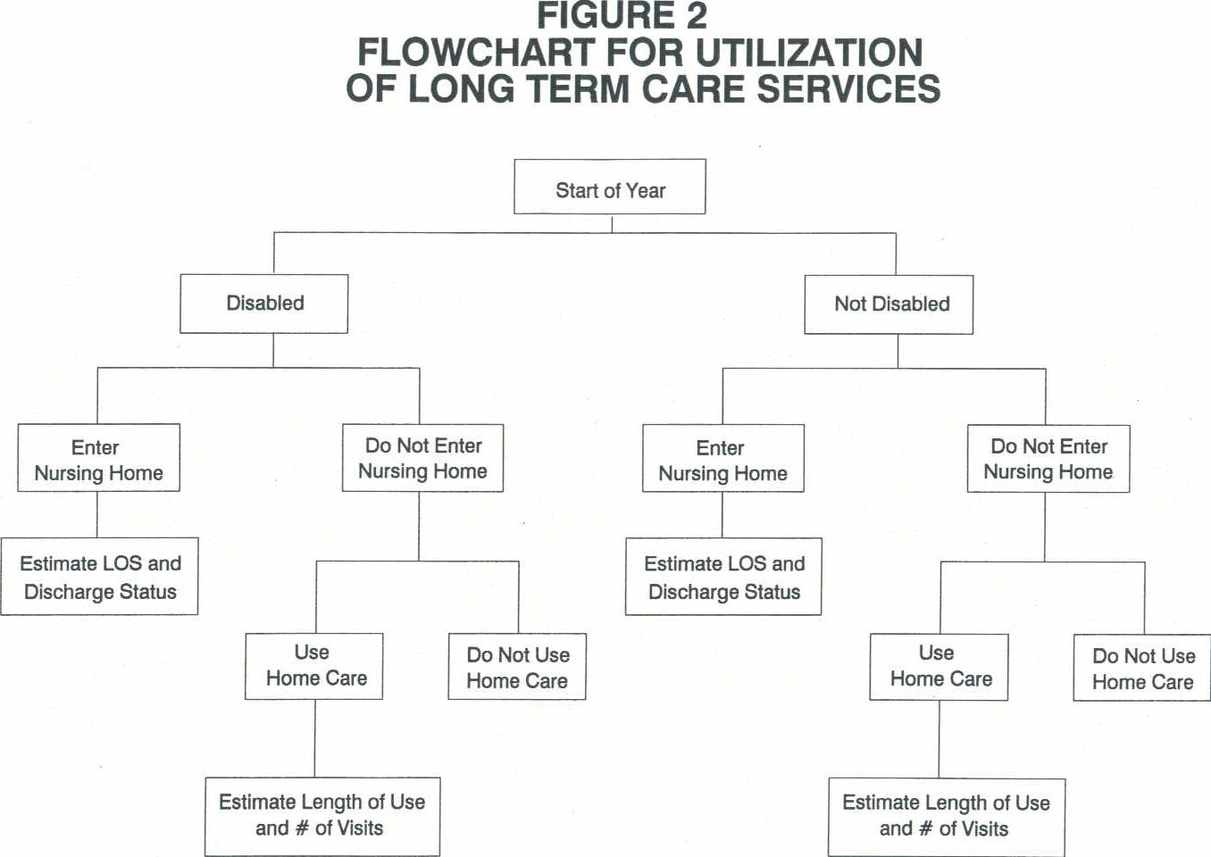
The probabilities used in the model implicitly assume that the rates of nursing home admission will remain constant over time on an age/sex/marital status basis for disabled and nondisabled persons. Constant rates imply that the nursing home bed supply will increase to accommodate admissions from an increasingly large elderly population. Rates can increase based on user-specified assumptions concerning induced demand.
The model only allows individuals to enter a nursing home once each year. This is reasonable assumption because the length of stay assumptions (discussed below) reflect an aggregation of lengths of stay for persons who were discharged from nursing homes and then reentered soon thereafter.
| TABLE 19. Annual Probability of Nursing Home Entry | ||||
| Persons with 2+ ADLs | ||||
| Age | Prior NursingHome Stay | No Prior NursingHome Stay | ||
| Single | Married | Single | Married | |
| 65 | 12.9% | 8.9% | 5.2% | 3.3% |
| 66 | 14.0% | 9.6% | 5.6% | 3.6% |
| 67 | 15.0% | 10.4% | 6.1% | 3.9% |
| 68 | 16.2% | 11.3% | 6.7% | 4.3% |
| 69 | 17.4% | 12.2% | 7.2% | 4.7% |
| 70 | 18.6% | 13.1% | 7.8% | 5.1% |
| 71 | 20.0% | 14.1% | 8.4% | 5.5% |
| 72 | 21.3% | 15.1% | 9.1% | 5.9% |
| 73 | 22.7% | 16.2% | 9.8% | 6.4% |
| 74 | 24.2% | 17.4% | 10.5% | 6.9% |
| 75 | 25.8% | 18.5% | 11.3% | 7.4% |
| 76 | 27.4% | 19.8% | 12.1% | 8.0% |
| 77 | 29.0% | 21.1% | 13.0% | 8.6% |
| 78 | 30.7% | 22.5% | 13.9% | 9.2% |
| 79 | 32.5% | 23.9% | 14.9% | 9.9% |
| 80 | 34.3% | 25.4% | 15.9% | 10.6% |
| 81 | 36.2% | 26.9% | 17.0% | 11.4% |
| 82 | 38.2% | 28.5% | 18.1% | 12.2% |
| 83 | 40.2% | 30.1% | 19.3% | 13.0% |
| 84 | 42.3% | 31.9% | 20.5% | 13.9% |
| 85 | 44.4% | 33.6% | 21.8% | 14.8% |
| 86 | 46.6% | 35.5% | 23.1% | 15.8% |
| 87 | 48.8% | 37.4% | 24.5% | 16.8% |
| 88 | 51.1% | 39.4% | 26.0% | 17.9% |
| 89 | 53.5% | 41.4% | 27.5% | 19.0% |
| 90 | 55.9% | 43.5% | 29.1% | 20.2% |
| 91 | 58.4% | 45.6% | 30.7% | 21.4% |
| 92 | 60.9% | 47.9% | 32.4% | 22.7% |
| 93 | 63.4% | 50.1% | 34.2% | 24.1% |
| 94 | 66.1% | 52.5% | 36.0% | 25.5% |
| 95 | 68.7% | 54.9% | 37.9% | 26.9% |
| 96 | 71.4% | 57.3% | 39.9% | 28.5% |
| 97 | 74.2% | 59.8% | 41.9% | 30.1% |
| 98 | 77.0% | 62.4% | 44.0% | 31.7% |
| 99 | 79.8% | 65.0% | 46.2% | 33.5% |
| 100 | 82.7% | 67.7% | 48.4% | 35.2% |
| SOURCE: Lewin-ICF and Brookings Institution calculations using data from the 1982-84 National Long Term Care Survey and the 1985 National Nursing Home Survey. | ||||
| TABLE 19. Annual Probability of Nursing Home Entry(continued) | ||||
| Persons with 1 ADL | ||||
| Age | Prior NursingHome Stay | No Prior NursingHome Stay | ||
| Single | Married | Single | Married | |
| 65 | 9.1% | 6.1% | 3.4% | 2.2% |
| 66 | 9.9% | 6.6% | 3.7% | 2.4% |
| 67 | 10.7% | 7.2% | 4.1% | 2.6% |
| 68 | 11.6% | 7.8% | 4.4% | 2.8% |
| 69 | 12.5% | 8.4% | 4.8% | 3.1% |
| 70 | 13.5% | 9.1% | 5.2% | 3.3% |
| 71 | 14.5% | 9.8% | 5.7% | 3.6% |
| 72 | 15.5% | 10.6% | 6.1% | 3.9% |
| 73 | 16.7% | 11.4% | 6.6% | 4.2% |
| 74 | 17.8% | 12.2% | 7.1% | 4.6% |
| 75 | 19.0% | 13.1% | 7.7% | 4.9% |
| 76 | 20.3% | 14.1% | 8.3% | 5.3% |
| 77 | 21.6% | 15.1% | 8.9% | 5.7% |
| 78 | 23.0% | 16.1% | 9.5% | 6.2% |
| 79 | 24.5% | 17.2% | 10.2% | 6.6% |
| 80 | 26.0% | 18.3% | 11.0% | 7.1% |
| 81 | 27.5% | 19.5% | 11.7% | 7.6% |
| 82 | 29.2% | 20.8% | 12.5% | 8.2% |
| 83 | 30.9% | 22.1% | 13.4% | 8.8% |
| 84 | 32.6% | 23.4% | 14.3% | 9.4% |
| 85 | 34.4% | 24.9% | 15.3% | 10.0% |
| 86 | 36.3% | 26.4% | 16.3% | 10.7% |
| 87 | 38.2% | 27.9% | 17.3% | 11.5% |
| 88 | 40.2% | 29.5% | 18.4% | 12.2% |
| 89 | 42.3% | 31.2% | 19.6% | 13.0% |
| 90 | 44.4% | 32.9% | 20.8% | 13.9% |
| 91 | 46.6% | 34.7% | 22.0% | 14.8% |
| 92 | 48.8% | 36.6% | 23.3% | 15.7% |
| 93 | 51.1% | 38.5% | 24.7% | 16.7% |
| 94 | 53.5% | 40.5% | 26.2% | 17.8% |
| 95 | 55.9% | 42.5% | 27.7% | 18.9% |
| 96 | 58.4% | 44.7% | 29.2% | 20.0% |
| 97 | 60.9% | 46.8% | 30.9% | 21.2% |
| 98 | 63.5% | 49.1% | 32.6% | 22.5% |
| 99 | 66.1% | 51.4% | 34.3% | 23.8% |
| 100 | 68.8% | 53.8% | 36.1% | 25.2% |
| SOURCE: Lewin-ICF and Brookings Institution calculations using data from the 1982-84 National Long Term Care Survey and the 1985 National Nursing Home Survey. | ||||
| TABLE 19. Annual Probability of Nursing Home Entry(continued) | ||||
| Persons with IADLs Only | ||||
| Age | Prior NursingHome Stay | No Prior NursingHome Stay | ||
| Single | Married | Single | Married | |
| 65 | 7.8% | 51.% | 2.9% | 1.8% |
| 66 | 8.5% | 5.6% | 3.1% | 2.0% |
| 67 | 9.2% | 6.1% | 3.4% | 2.2% |
| 68 | 10.0% | 6.6% | 3.7% | 2.3% |
| 69 | 10.8% | 7.2% | 4.1% | 2.6% |
| 70 | 11.6% | 7.8% | 4.4% | 2.8% |
| 71 | 12.5% | 8.4% | 4.8% | 3.0% |
| 72 | 13.5% | 9.0% | 5.2% | 3.3% |
| 73 | 14.4% | 9.7% | 5.6% | 3.5% |
| 74 | 15.5% | 10.5% | 6.0% | 3.8% |
| 75 | 16.6% | 11.3% | 6.5% | 4.1% |
| 76 | 17.7% | 12.1% | 7.0% | 4.5% |
| 77 | 18.9% | 12.9% | 7.5% | 4.8% |
| 78 | 20.1% | 13.9% | 8.1% | 5.2% |
| 79 | 21.5% | 14.8% | 8.7% | 5.6% |
| 80 | 22.8% | 15.8% | 9.3% | 6.0% |
| 81 | 24.2% | 16.9% | 10.0% | 6.4% |
| 82 | 25.7% | 18.0% | 10.7% | 6.9% |
| 83 | 27.3% | 19.2% | 11.4% | 7.4% |
| 84 | 28.9% | 20.4% | 12.2% | 7.9% |
| 85 | 30.5% | 21.6% | 13.0% | 8.5% |
| 86 | 32.2% | 23.0% | 13.9% | 9.1% |
| 87 | 34.0% | 24.4% | 14.8% | 9.7% |
| 88 | 35.9% | 25.8% | 15.8% | 10.4% |
| 89 | 37.8% | 27.3% | 16.8% | 11.1% |
| 90 | 39.8% | 28.9% | 17.8% | 11.8% |
| 91 | 41.8% | 30.5% | 19.0% | 12.6% |
| 92 | 43.9% | 32.2% | 20.1% | 13.4% |
| 93 | 46.1% | 34.0% | 21.4% | 14.3% |
| 94 | 48.3% | 35.8% | 22.6% | 15.2% |
| 95 | 50.6% | 37.7% | 24.0% | 16.1% |
| 96 | 52.9% | 39.7% | 25.4% | 17.1% |
| 97 | 55.3% | 41.7% | 26.8% | 18.2% |
| 98 | 57.8% | 43.8% | 28.4% | 19.3% |
| 99 | 60.3% | 46.0% | 29.9% | 20.4% |
| 100 | 62.9% | 48.2% | 31.6% | 21.7% |
| SOURCE: Lewin-ICF and Brookings Institution calculations using data from the 1982-84 National Long Term Care Survey and the 1985 National Nursing Home Survey. | ||||
| TABLE 19. Annual Probability of Nursing Home Entry(continued) | ||||||||
| Non-Disabled Persons | ||||||||
| Age | Prior NursingHome Stay | No Prior NursingHome Stay | ||||||
| Males | Females | Males | Females | |||||
| Single | Married | Single | Married | Single | Married | Single | Married | |
| 65 | 7.9% | 3.0% | 6.0% | 2.2% | 0.6% | 0.2% | 0.4% | 0.1% |
| 66 | 9.1% | 3.5% | 7.0% | 2.6% | 0.7% | 0.2% | 0.5% | 0.2% |
| 67 | 10.4% | 4.1% | 8.0% | 3.0% | 0.8% | 0.3% | 0.6% | 0.2% |
| 68 | 11.8% | 4.7% | 9.2% | 3.5% | 0.9% | 0.3% | 0.7% | 0.2% |
| 69 | 13.4% | 5.4% | 10.4% | 4.0% | 1.1% | 0.4% | 0.8% | 0.3% |
| 70 | 15.2% | 6.2% | 11.9% | 4.7% | 1.3% | 0.4% | 0.9% | 0.3% |
| 71 | 17.1% | 7.2% | 13.5% | 5.4% | 1.5% | 0.5% | 1.1% | 0.4% |
| 72 | 19.2% | 8.2% | 15.2% | 6.2% | 1.7% | 0.6% | 1.2% | 0.4% |
| 73 | 21.4% | 9.3% | 17.1% | 7.1% | 2.0% | 0.7% | 1.4% | 0.5% |
| 74 | 23.8% | 10.6% | 19.2% | 8.1% | 2.3% | 0.8% | 1.7% | 0.6% |
| 75 | 26.4% | 12.1% | 21.4% | 9.2% | 2.6% | 0.9% | 1.9% | 0.7% |
| 76 | 29.2% | 13.6% | 23.9% | 10.5% | 3.0% | 1.0% | 2.2% | 0.8% |
| 77 | 32.1% | 15.4% | 26.5% | 11.9% | 3.5% | 1.2% | 2.5% | 0.9% |
| 78 | 35.2% | 17.3% | 29.3% | 13.4% | 4.0% | 1.4% | 2.9% | 1.0% |
| 79 | 38.4% | 19.4% | 32.2% | 15.2% | 4.5% | 1.6% | 3.3% | 1.2% |
| 80 | 41.8% | 21.7% | 35.3% | 17.1% | 5.2% | 1.8% | 3.8% | 1.3% |
| 81 | 45.3% | 24.1% | 38.6% | 19.1% | 5.9% | 2.1% | 4.4% | 1.5% |
| 82 | 49.0% | 26.8% | 42.1% | 21.4% | 6.8% | 2.4% | 5.0% | 1.8% |
| 83 | 52.7% | 29.7% | 45.7% | 23.8% | 7.7% | 2.8% | 5.8% | 2.0% |
| 84 | 56.6% | 32.7% | 49.4% | 26.5% | 8.8% | 3.2% | 6.6% | 2.3% |
| 85 | 60.6% | 35.9% | 53.3% | 29.3% | 10.0% | 3.6% | 7.5% | 2.7% |
| 86 | 60.6% | 35.9% | 53.3% | 29.3% | 11.3% | 4.2% | 8.5% | 3.1% |
| 87 | 60.6% | 35.9% | 53.3% | 29.3% | 12.8% | 4.8% | 9.6% | 3.5% |
| 88 | 60.6% | 35.9% | 53.3% | 29.3% | 14.4% | 5.4% | 10.9% | 4.0% |
| 89 | 60.6% | 35.9% | 53.3% | 29.3% | 16.2% | 6.2% | 12.4% | 4.6% |
| 90 | 60.6% | 35.9% | 53.3% | 29.3% | 18.2% | 7.0% | 13.9% | 5.2% |
| 91 | 60.6% | 35.9% | 53.3% | 29.3% | 20.4% | 8.0% | 15.7% | 5.9% |
| 92 | 60.6% | 35.9% | 53.3% | 29.3% | 22.8% | 9.1% | 17.6% | 6.7% |
| 93 | 60.6% | 35.9% | 53.3% | 29.3% | 35.4% | 10.3% | 19.8% | 7.7% |
| 94 | 60.6% | 35.9% | 53.3% | 29.3% | 28.2% | 11.6% | 22.1% | 8.7% |
| 95 | 60.6% | 35.9% | 53.3% | 29.3% | 31.3% | 13.1% | 24.7% | 9.9% |
| 96 | 60.6% | 35.9% | 53.3% | 29.3% | 34.5% | 14.8% | 27.4% | 11.1% |
| 97 | 60.6% | 35.9% | 53.3% | 29.3% | 38.0% | 16.6% | 30.4% | 12.6% |
| 98 | 60.6% | 35.9% | 53.3% | 29.3% | 41.8% | 18.7% | 33.7% | 14.2% |
| 99 | 60.6% | 35.9% | 53.3% | 29.3% | 45.7% | 20.9% | 37.1% | 16.0% |
| 100 | 60.6% | 35.9% | 53.3% | 29.3% | 49.8% | 23.4% | 40.8% | 17.9% |
| SOURCE: Lewin-ICF and Brookings Institution calculations using data from the 1982-84 National Long Term Care Survey and the 1985 National Nursing Home Survey. | ||||||||
2. Nursing Home Length of Stay and Discharge Status
Individuals who are simulated to enter nursing homes are assigned a length of stay and a discharge status (alive or dead) based upon their age and marital status at entry. These length of stay probabilities are shown in Table 20 and are based upon lengths of stay developed from the 1985 National Nursing Home Survey Discharge File. These probabilities implicitly assume that age-group/marital status specific lengths of stay in nursing homes do not change after 1985.
There is no data set that records admissions to a nursing home and nursing home length of stay on a national basis. The 1985 National Nursing Home Survey (NNHS) is the best nationally representative data base on nursing home use, but only has a current resident survey and a discharge survey. The current resident survey reflects an average daily census for nursing homes in the U.S. The discharge survey is a sample of all the discharges from nursing homes in a year.
The 1985 National Nursing Home Discharge File was used to determine nursing home length of stay and to create a synthetic admission cohort. The synthetic admission cohort is intended to accurately represent the population entering nursing homes in 1985 by adjusting discharges for duplicate counting of individuals with more than one nursing home discharge and adjusting for the growth in the bed supply.
For the 1985 NNHS discharge file to accurately reflect an admission cohort, rather than all discharges during the year, three major problems with the NNHS Discharge File had to be addressed:
-
First, the file reflects discharges not persons; because the model simulates utilization by persons, the discharges must be related to persons;
-
Second, for persons with multiple discharges (i.e., discharged from one nursing home and admitted to another, or discharged from a nursing home to a hospital and then readmitted to a nursing home) the length of stay on the file does not represent the true length of stay. Because the model simulates total length of stay within any one episode of care, the multiple discharges need to be aggregated for each individual; and
-
Third, in converting discharges to admissions it is necessary to take into account the effect of changes in the supply of nursing home beds over time on the number of long stays. This must be done to accurately reflect the likelihood of a person entering a nursing home in 1985 (if an adjustment for increases in bed supply was not made the probabilities would reflect the likelihood of entry when the bed supply was smaller).
| TABLE 20. The Probability of Nursing Home Length of Stay by Age of Entry and Marital Statusa,b | ||||||
| Length of Stay(in days) | Age of Entry | |||||
| 65-74 | 75-84 | 85+ | ||||
| Live | Dead | Live | Dead | Live | Dead | |
| MARRIED | ||||||
| 1-29 | 21.04% | 14.64% | 17.25% | 23.46% | 16.30% | 17.14% |
| 30-59 | 3.91% | 9.76% | 8.99% | 7.09% | 7.95% | 5.73% |
| 60-89 | 2.09% | 2.48% | 1.76% | 2.85% | 3.24% | 3.67% |
| 90-179 | 6.61% | 8.27% | 3.10% | 4.58% | 1.59% | 5.26% |
| 180-273 | 3.63% | 3.07% | 1.92% | 5.17% | 1.17% | 3.61% |
| 274-364 | 0.83% | 0.74% | 0.37% | 2.78% | 0.00% | 3.01% |
| 365-547 | 0.81% | 2.36% | 0.56% | 3.92% | 2.19% | 4.88% |
| 548-729 | 0.32% | 2.24% | 0.14% | 3.58% | 0.31% | 1.60% |
| 730-1,094 | 0.69% | 4.74% | 0.32% | 3.79% | 4.23% | 4.01% |
| 1,095-1,469 | 0.20% | 2.15% | 0.82% | 1.68% | 0.00% | 1.07% |
| 1,470-1,824 | 0.67% | 2.89% | 0.36% | 1.08% | 1.35% | 3.74% |
| 1,825-2,189 | 0.16% | 2.50% | 0.00% | 1.66% | 0.22% | 1.71% |
| 2,190+ | 0.05% | 3.19% | 0.39% | 2.37% | 0.76% | 5.25% |
| Total | 40.96% | 59.02% | 35.99% | 64.01% | 39.33% | 60.67% |
| UNMARRIED | ||||||
| 1-29 | 16.85% | 8.21% | 13.53% | 9.67% | 10.77% | 11.73% |
| 30-59 | 8.89% | 2.93% | 5.51% | 5.48% | 5.33% | 5.47% |
| 60-89 | 4.81% | 2.52% | 3.51% | 2.99% | 2.09% | 3.89% |
| 90-179 | 5.53% | 4.84% | 5.05% | 4.16% | 4.01% | 7.07% |
| 180-273 | 2.81% | 2.46% | 1.98% | 4.37% | 0.74% | 3.93% |
| 274-364 | 1.77% | 1.53% | 1.82% | 2.15% | 1.01% | 4.08% |
| 365-547 | 1.91% | 4.09% | 1.43% | 5.24% | 1.72% | 4.49% |
| 548-729 | 1.44% | 2.91% | 0.79% | 4.67% | 0.64% | 4.21% |
| 730-1,094 | 0.45% | 5.03% | 1.70% | 5.32% | 0.80% | 7.40% |
| 1,095-1,469 | 0.84% | 4.16% | 0.94% | 4.54% | 0.79% | 4.87% |
| 1,470-1,824 | 0.87% | 1.60% | 0.76% | 3.86% | 0.55% | 4.21% |
| 1,825-2,189 | 0.56% | 1.70% | 0.49% | 2.54% | 0.06% | 2.25% |
| 2,190+ | 1.03% | 10.24% | 0.60% | 6.91% | 0.89% | 7.03% |
| Total | 47.78% | 52.22% | 38.10% | 61.90% | 29.37% | 70.63% |
SOURCE: Brookings Institution and Lewin-ICF calculations using data from 1985 National Nursing Home Survey. | ||||||
Conversion from discharges to discharged persons -- Some persons are discharged more than once in the same year. To avoid double counting, the discharge file was converted to a file of persons. In converting from discharges to persons, the last discharge during the year was assumed to be the "reference" discharge for each person. Alternatively, the first discharge in the survey year could have been used. Both methods are equally valid, but using the last discharge provides more accurate length of stay data because it allows a more accurate aggregation of discharges which have occurred previously. Specifically, in converting the file of discharges to discharged persons, two types of discharges were eliminated:
-
persons who had a subsequent discharge within the survey year (to avoid double counting); and
-
all discharges for individuals who had a subsequent nursing home admission within 30 days of the surveyed discharge (these individuals would either have another discharge during the survey year and therefore would be double counted or have a discharge outside the survey year and should not be included in the 1985 admission cohort).
For example, if a discharge on the Discharge File reported a subsequent discharge within the survey year, this discharge was not included in our admission cohort. With the exception of the two situations described above, all discharges were included in the admission cohort. After converting from elderly discharges to persons, the number of discharges on the 1985 NNHS file was reduced from 1,090,400 to 801,400.
Length of stay -- Although the length of stay for the reference nursing home discharge is complete, it does not capture total length of stay for persons with previous discharges. The NNHS records information on previous stays and discharge destinations. Therefore, for those with previous discharges and a re-admission within 30 days of discharge, the actual previous lengths of stay were added to the reference length of stay. The prior lengths of stay were estimated directly from the file except in two cases:
-
First, for persons who report more than two previous stays, an additional third previous stay was simulated.19 Because the length of this third previous stay was unknown, a length of stay was randomly assigned. This length of stay was based on the distribution of 1985 discharges which had a subsequent nursing home admission within 30 days of discharge but no previous stay. These discharges best approximated the length of stay of persons with a third previous stay.
-
Second, an additional previous stay was imputed to persons admitted directly from another nursing home to their "reference" discharge stay where length of stay data was unavailable for their previous stay. The length of stay distribution used was the same as for the first adjustment.
Cohort effect -- The 801,400 discharged persons were further adjusted to reflect the cohort effect of the growth in the nursing home bed supply. The discharge survey undercounts the number of people with long lengths of stay because there were fewer nursing home beds when people with long stays were admitted, and thus, fewer people could be admitted. Therefore, the number of people in each length of stay group was increased using a growth factor calculated from the total increase in nursing home residents from 1977 to 1985 (1.402 to 1.624 million). For example, the one to two year category was adjusted by the estimated growth in the number of beds between 1984 and 1985, the two to three year category was adjusted by the estimated growth in beds from 1983 to 1985, and so on. After this adjustment, the total number of adjusted admissions for 1985 was 824,600.
In the model, nursing home entrants are assigned a number of days within the length of stay range to which they are assigned so that the expected cross-section estimate is approximated (see Table 21).
| TABLE 21. Number of Nursing Home Days Assigned by Length of Stay Category | |
| Length of Stay Category | Number of Days Assigned |
| 30 Days | 14 |
| 1-2 Months | 42 |
| 2-3 Months | 73 |
| 3-6 Months | 129 |
| 6-9 Months | 220 |
| 9-12 Months | 314 |
| 1-1.5 Years | 452 |
| 1.5-2 Years | 634 |
| 2-3 Years | 898 |
| 3-4 Years | 1,257 |
| 4-5 Years | 1,626 |
| 5-6 Years | 1,988 |
| 6+ Years | 3,619 |
| SOURCE: Brookings Institution and Lewin-ICF calculations using data from the 1985 National Nursing Home Survey. | |
3. Disability Level in the Nursing Home
Once an individual enters a nursing home, the model assigns the individual a nursing home disability level. The model assigns these disability levels because the disability status of an individual can change from the beginning of the year to the time when he or she enters a nursing home. The nursing home disability prevalence rates in Table 22 are based on the 1985 National Nursing Home Survey Current Resident File.20 The disability levels vary by age and marital status. Individuals with two or more ADLs prior to entry are assumed to continue to have this level of disability. Individuals with lesser disabilities are assumed to have an increase in disability so that the distribution of disability of residents in the model matches the distribution of disability among residents in the 1985 NNHS. When nursing home disability status is assigned, the disability status of an individual can only increase, i.e., people's conditions do not improve at the point of entry to a nursing home.
4. Nursing Home Discharge Level of Disability
When an individual is discharged alive, he or she is then assigned a new disability level. The discharge disability level prevalence rates vary by length of stay. The prevalence rates in Table 23 were developed from the 1985 NNHS Discharge File, based on people discharged alive to the community. These people have relatively few disabilities compared to current residents because they are being discharged to home.
The 1985 NNHS Discharge File only has disability variables indicating deficiencies in mobility or continence. To categorize individuals using the three disability levels in the model, we assumed discharged residents with no deficiency in either mobility or continence were in the IADL only category; residents with a deficiency in either mobility or continence fell into the one ADL category; and residents with deficiencies in both mobility and continence were considered to have two or more ADLs.
5. Induced Demand
The model can simulate an increase in nursing home use as a result of changes in financing mechanisms. This increased use is often referred to as moral hazard or induced demand. Estimates of induced demand reflect additional admissions or increased lengths of stay as a result of new third-party payment sources.
| TABLE 22. Nursing Home Disability Prevalence Rates | ||||||
| IADL Onlya | 1 ADL | 2+ ADLs | ||||
| Married | Unmarried | Married | Unmarried | Married | Unmarried | |
| 65-69 | 7.8% | 18.6% | 6.8% | 19.1% | 85.5% | 62.3% |
| 70-74 | 5.6 | 13.4 | 8.7 | 14.6 | 85.7 | 72.1 |
| 75-79 | 5.3 | 11.4 | 9.3 | 13.5 | 85.4 | 75.0 |
| 80-84 | 7.9 | 8.0 | 5.6 | 14.0 | 86.5 | 78.0 |
| 85-89 | 3.6 | 6.4 | 10.1 | 11.3 | 86.3 | 82.2 |
| 90+ | 3.5 | 4.5 | 2.3 | 10.6 | 94.2 | 84.9 |
SOURCE: Brookings Institution and Lewin-ICF assumptions based upon data from the 1985 National Nursing Home Survey Current Resident File. | ||||||
| TABLE 23. Nursing Home Discharge Disability Prevalence Rate | ||
| Length of Stay | ||
| Less than 3 Months | More Than 3 Months | |
| IADL Onlya | 52.2% | 40.1% |
| 1 ADL | 25.8 | 26.1 |
| 2+ ADLs | 21.9 | 33.8 |
| Total | 100.0% | 100.0% |
SOURCE: Brookings Institution and Lewin-ICF calculations using data from 1985 National Nursing Home Survey Discharge File. | ||
The model can estimate the effects of a given level of induced demand (user specified) by simulating additional nursing home admissions. The model assumes these admissions are based upon the same pattern of nursing home admissions reflected in the entry probabilities in Table 19. For example, if a new public program is expected to increase nursing home entries by ten percent, the probabilities in Table 19 would be multiplied by 0.1, and those persons who had not entered a nursing home as a result of the base case probabilities would be subjected to the additional probability of nursing home entrance. These new admissions are then financed by the proposed program or simulated insurance policy. Of course, only persons who meet the requirements of the program or with insurance would enter the nursing home under the induced demand probabilities.21
Individuals who enter a nursing home due to induced demand are assumed to have the length of stay probabilities shown in Table 24. These probabilities are based upon data from the 1985 NNHS. The disability status and mortality probabilities of individuals who enter a nursing home due to induced demand remains the same as in the base case.
B. Home Care Utilization
Some individuals age 65 and over are simulated to use home care services. These services include home health care, homemaker, chore, personal care, and meal preparation services.
As shown in Figure 3, the model simulates the use of home care services for a number of distinct groups of the elderly:
-
First, the model determines whether an individual is chronically disabled at the start of the year or whether the individual becomes chronically disabled during the year. (See Section III on disability);
-
Second, the model determines which chronically disabled persons and persons not chronically disabled at the start of the year use formal (paid) home care services;
-
Third, the model determines the number of visits received and the period of use for users.
-
Fourth, for individuals using home care, the model then determines if any visits are Medicare-covered home health services;
-
Fifth, the model determines which nonchronically disabled persons receive Medicare home health services;
| TABLE 24. The Probability of Nursing Home Length of Stay by Age of Entry and Marital Status for Persons Using Services Due to Induced Demanda | |||
| Length of Stay(in days) | Age of Entry | ||
| 65-74 | 75-84 | 85+ | |
| MARRIED | |||
| 1-29 | 28.6% | 32.3% | 29.5% |
| 30-59 | 13.1 | 14.0 | 13.6 |
| 60-89 | 7.8 | 5.4 | 5.1 |
| 90-179 | 14.3 | 9.6 | 9.1 |
| 180-364 | 11.1 | 9.1 | 10.0 |
| 365-729 | 8.2 | 9.9 | 10.4 |
| 730-1,094 | 5.5 | 4.4 | 5.3 |
| 1,095-1,469 | 3.2 | 2.8 | 4.3 |
| 1,470-1,824 | 2.7 | 2.4 | 4.7 |
| 1,825-2,189 | 1.6 | 3.1 | 1.8 |
| 2,190+ | 3.9 | 7.0 | 6.2 |
| Total | 100.0% | 100.0% | 100.0% |
| UNMARRIED | |||
| 1-29 | 21.2% | 19.7% | 19.3% |
| 30-59 | 11.7 | 10.7 | 9.5 |
| 60-89 | 7.0 | 5.4 | 5.5 |
| 90-179 | 9.6 | 9.8 | 11.5 |
| 180-364 | 9.1 | 12.1 | 11.8 |
| 365-729 | 9.1 | 10.8 | 13.2 |
| 730-1,094 | 7.1 | 7.2 | 7.5 |
| 1,095-1,469 | 4.0 | 6.3 | 5.8 |
| 1,470-1,824 | 2.5 | 4.4 | 4.3 |
| 1,825-2,189 | 3.3 | 3.3 | 2.7 |
| 2,190+ | 15.4 | 10.3 | 8.9 |
| Total | 100.0% | 100.0% | 100.0% |
SOURCE: Brookings Institution and Lewin-ICF calculations using data from the 1985 National Nursing Home Survey. | |||
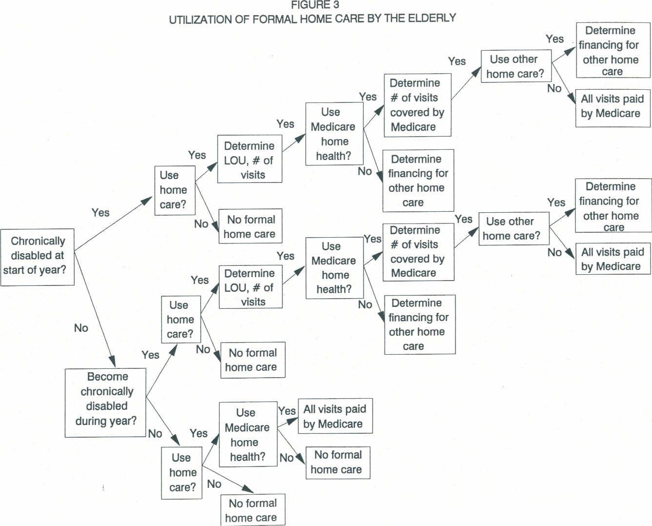
The model assumes that persons in a nursing home do not use home care services while they are in a nursing home. Persons using nursing home services for part of the year may also use home care services.
1. Probability of Starting to Use Home Care for the Chronically Disabled
As discussed above and as shown in Figure 3, three groups of the elderly are simulated by the model to start using home care services in each year: 1) some persons who were chronically disabled at the start of the year; 2) some persons who were not chronically disabled at the start of the year but who become chronically disabled during the year; and 3) some persons who are not chronically disabled but use Medicare home health services as part of their recovery from an acute illness. The likelihood of starting to use home care services was estimated for each of these groups separately.
The likelihood of starting to use services was estimated from two data sources: 1) the 1982-84 NLTCS; and 2) Medicare program data. The 1982-84 NLTCS permits estimates of the likelihood of starting to use services for the chronically disabled; Medicare program data allows one to estimate use among the nonchronically disabled.
The 1982-84 NLTCS reports the characteristics of persons in 1982 and whether or not they used services in 1984. Unfortunately, in contrast to data in the NLTCS on nursing home use, the NLTCS does not allow one to know whether an individual used services at anytime during the 1982-84 period. Rather, it only indicates if services were being used at the time of the interview in 1984. As a consequence, the likelihood of using services in 1984 had to be estimated based upon the characteristics of individuals in 1982. These probabilities then had to be adjusted to account for persons who used services during the year but who were not receiving services on the day of the survey interview.
Separate logistic regression equations were estimated for: 1) noninstitutionalized persons who were chronically disabled in 1982; and 2) noninstitutionalized persons who were not chronically disabled in 1982 but who were chronically disabled in 1984. The equations for the noninstitutionalized disabled were estimated as a function of disability level and sex. Surprisingly, age and marital status were not significant at the 95 percent confidence level. The equation for the nondisabled was estimated as a function of age, sex, and marital status.
These equations allowed us to estimate the probability of using services in 1984 given one's characteristics in 1982 for persons who were either chronically disabled in 1982 or became chronically disabled during the 1982-84 period. However, in the model we want to simulate the start or incidence of use of services. Incidence rates were approximated using the cross-sectional data by assuming that the incidence rate was equal to the prevalence rate divided by the reported duration of use for each group of users. For example, if all users of home care in the survey had been using services for a period of two years, the incidence rate would be estimated as one-half the prevalence rate.
| TABLE 25. Annual Probability of Starting to Use Formal Home Care Services for the Noninstitutionalized Chronically Disabled | ||
| Disability Level | Males | Females |
| IADL Only | 12.9% | 22.0% |
| 1 ADL | 15.9 | 26.6 |
| 2+ ADLs | 16.6 | 27.7 |
| SOURCE: Brookings Institution and Lewin-ICF estimates based upon analysis of the 1982-84 National Long Term Care Survey. | ||
| TABLE 26. Annual Probability of Starting to Use Formal Home Care for Persons Who are Noninstitutionalized and Nondisabled at the Start of the Year | ||||
| Age | Males | Females | ||
| Married | Single | Married | Single | |
| 65 | 1.56% | 0.92% | 2.14% | 1.26% |
| 66 | 1.69 | 0.99 | 2.31 | 1.37 |
| 67 | 1.82 | 1.07 | 2.50 | 1.48 |
| 68 | 1.97 | 1.16 | 2.70 | 1.59 |
| 69 | 2.12 | 1.25 | 2.91 | 1.72 |
| 70 | 2.29 | 1.35 | 3.14 | 1.86 |
| 71 | 2.48 | 1.46 | 3.39 | 2.01 |
| 72 | 2.67 | 1.58 | 3.66 | 2.17 |
| 73 | 2.89 | 1.71 | 3.95 | 2.34 |
| 74 | 3.12 | 1.85 | 4.26 | 2.53 |
| 75 | 3.36 | 1.99 | 4.59 | 2.73 |
| 76 | 3.63 | 2.15 | 4.95 | 2.95 |
| 77 | 3.91 | 2.32 | 5.33 | 3.18 |
| 78 | 4.22 | 2.51 | 5.75 | 3.43 |
| 79 | 4.55 | 2.71 | 6.19 | 3.71 |
| 80 | 4.91 | 2.92 | 6.67 | 4.00 |
| 81 | 5.29 | 3.16 | 7.18 | 4.31 |
| 82 | 5.70 | 3.41 | 7.73 | 4.65 |
| 83 | 6.14 | 3.68 | 8.31 | 5.01 |
| 84 | 6.61 | 3.96 | 8.94 | 5.40 |
| 85 | 7.12 | 4.28 | 9.61 | 5.82 |
| 86 | 7.66 | 4.61 | 10.33 | 6.27 |
| 87 | 8.25 | 4.97 | 11.09 | 6.75 |
| 88 | 8.87 | 5.36 | 11.91 | 7.27 |
| 89 | 9.53 | 5.77 | 12.78 | 7.82 |
| 90 | 10.25 | 6.22 | 13.70 | 8.42 |
| 91 | 11.01 | 6.70 | 14.68 | 9.05 |
| 92 | 11.81 | 7.21 | 15.72 | 9.73 |
| 93 | 12.68 | 7.76 | 16.83 | 10.46 |
| 94 | 13.59 | 8.35 | 18.00 | 11.23 |
| 95 | 14.57 | 8.98 | 19.23 | 12.05 |
| 96 | 15.61 | 9.65 | 20.54 | 12.93 |
| 97 | 16.70 | 10.37 | 21.91 | 13.86 |
| 98 | 17.86 | 11.14 | 23.35 | 14.86 |
| 99 | 19.09 | 11.96 | 24.87 | 15.91 |
| 100 | 20.39 | 12.83 | 26.46 | 17.02 |
| SOURCE: Brookings Institution and Lewin-ICF estimates based on data from the 1982-84 National Long Term Care Survey. | ||||
The logit equations discussed above allowed the estimation of the prevalence rates. Prevalence rates were divided by the reported duration of use in the 1984 NLTCS to produce estimates of incidence. This procedure underestimated the number of users in 1984 by 23 percent. As a consequence, the incidence rates were multiplied by a factor of 1.23. The adjusted probabilities of starting to use home care for the chronically disabled are shown in Table 25 and Table 26. Table 25 shows estimates for persons who are disabled at the start of the year. Table 26 provides estimates for persons who are not disabled at the start of the year but who become disabled during the course of the year.
Once a chronically disabled individual is selected to receive paid home care, he or she is then assigned a disability status for the duration of his or her home care use. The disability level rates for home care users were estimated with data on users of paid home care from the 1984 NLTCS. The prevalence rates were computed as the proportion of persons in each of the disability/age/marital status groups who reported receiving paid home care on the 1984 NLTCS. Table 27 presents the paid home care disability level prevalence rates for the chronically disabled users.
2. Duration and Intensity of Service Use by the Chronically Disabled
Once the model simulates the number of chronically disabled elderly individuals who receive home care services and assigns each of them a home care disability level, it determines how long and how often they will receive home care. Disabled home care recipients' length of use was estimated from the 1982-84 NLTCS adjusted for extended episodes of home care22 (Table 28).
Once the number of months of formal home care utilization is assigned for each individual, the model estimates the number of home care visits per month based upon the disability level assigned to formal home care users. Table 29 shows these probabilities, which were estimated from the 1984 NLTCS. The model assumes that individuals in the 1-10 visits category receive 7 visits; individuals in the 11-20 visits category receive 15 visits; and persons in the 21+ visits category receive 32 visits per month.
The length of formal or informal home care use assigned to an individual may be modified by the model in two instances. First, use of home care services terminates when an individual is simulated to die. Second, use of home care also terminates upon entering a nursing home. For example, assume an individual is assigned a three year period of home care use starting in 1988 and terminating at the end of 1990 and that in 1989 the model simulates that the individual enters a nursing home for 45 days. In this instance, the individual would receive 365 days of home care in 1988. However, home care services would terminate in 1989 when the individual enters the nursing home. Thus, home care utilization in 1989 would be only 320 days (i.e., 365 less 45 days in an institution). Services would not continue into 1990. These rules apply to both formal and informal home care.
| TABLE 27. Disability Level Prevalence Rates for Chronically Disabled Users of Paid Home Care | ||||||
| Married | Unmarried | |||||
| 65-74 | 75-84 | 85+ | 65-74 | 75-84 | 85+ | |
| IADL Only | 25.2 | 23.9 | 16.7 | 34.1 | 32.3 | 33.9 |
| 1 ADL | 18.5 | 20.9 | 16.7 | 24.3 | 25.6 | 37.8 |
| 2+ ADLs | 56.3 | 55.2 | 66.6 | 41.6 | 42.1 | 28.3 |
| Total | 100.0% | 100.0% | 100.0% | 100.0% | 100.0% | 100.0% |
| SOURCE: Brookings Institution and Lewin-ICF calculations using 1982-84 NLTCS. | ||||||
| TABLE 28. Distribution of Home Care Length of Use for the Chronically Disabled | ||
| Duration | PercentageDistribution | Assigend Number ofMonths of Use |
| Less than 3 months | 59.0% | 2.0 |
| 3-6 months | 14.2 | 4.5 |
| 6-12 months | 9.6 | 9.0 |
| 12-36 months | 7.1 | 24.0 |
| 36-60 months | 7.0 | 48.0 |
| More than 60 months | 3.1 | 72.0 |
| Total | 100.0% | |
| SOURCE: Brookings Institution and Lewin-ICF calculations using data from the 1982-84 NLTCS. | ||
| TABLE 29. Monthly Number of Formal Visits by Formal Home Care Disability Levela | |||
| Monthly Numberof Visits | Formal Home Care Disability | ||
| IADL Only | 1 ADL | 2+ ADLs | |
| 1-10 | 69.9% | 59.1% | 38.7% |
| 11-20 | 8.4 | 8.0 | 11.8 |
| 21+ | 21.7 | 32.9 | 49.5 |
| Total | 100.0% | 100.0% | 100.0% |
SOURCE: Brookings Institution and Lewin-ICF calculations using data from 1982-1984 National Long Term Care Survey. | |||
Upon termination of an assigned length of home care use, an individual may again be selected to receive home care using the probabilities presented in Table 25, Table 26 and Table 31. This is also true for all individuals, including those who were discharged alive from a nursing home in a prior year. This implicitly assumes that the probability of home care utilization is the same for all individuals regardless of the individual's home care or nursing home utilization in prior years.
3. Use of Medicare Home Health Services
Some chronically disabled home care users, as well as some non- disabled persons recovering from acute illnesses, are simulated to receive Medicare home health service.
Chronically Disabled -- Based upon an analysis of the 1984 NLTCS, we estimate that 41.4 percent of the chronically disabled elderly receiving paid home care received Medicare reimbursement for some or all of their paid home care visits.
For the 41.4 percent of chronically disabled elderly home care users selected, the model then simulates the maximum number of visits covered by Medicare. Table 30 shows the probabilities of having a certain number of visits reimbursed by Medicare for persons receiving Medicare home health services. The actual number of visits covered in the model is are also shown in Table 30. The probabilities are based on Health Care Financing Administration (HCFA) data from the Medicare statistical system on the number of persons served by Medicare and the number of visits received.
| TABLE 30. Medicare Reimbursed Home Health Visits | ||
| Number ofReimbursed Visits | Assigned Visits | Probability |
| 1-9 | 6 | 39.9% |
| 10-20 | 16 | 23.3 |
| 21-30 | 27 | 12.1 |
| 31-40 | 38 | 7.1 |
| 41-50 | 49 | 4.6 |
| 51-99 | 82 | 8.5 |
| 100+ | 165 | 4.1 |
| 100.0% | ||
| SOURCE: Brookings Institution and Lewin-ICF calculations using Health Care Financing Administration data from the Medicare statistical system. | ||
If the total number of visits assigned by the model for these Medicare users is less than the maximum number covered by Medicare, all paid home care is reimbursed by Medicare. If the total number of visits is greater than the maximum number of visits covered by Medicare, the remaining visits are financed out-of-pocket, by other payers or by Medicaid.23 For example, if an individual is allowed 15 visits reimbursed by Medicare and is assigned a length of use for paid home care of less than three months, he or she would have 19 visits remaining after the Medicare reimbursed visits ((two months of use times 17 visits per month) -- (15 maximum covered by Medicare) = 19).
Nonchronically Disabled -- Comparison of Medicare program data and the 1984 National Long Term Care Survey data suggests that many individuals who receive Medicare home health visits are not chronically disabled and thus not included in the NLTCS sample. In order for the model simulations to agree with Medicare Program data, separate Medicare home health care use probabilities were estimated for the nonchronically disabled elderly. These probabilities, shown in Table 31, are applied to all nondisabled elderly persons who were not selected to receive paid home care with the previous set of probabilities.
If a nonchronically disabled elderly individual is selected to receive Medicare home health visits, he or she is assigned a number of visits based on probabilities shown in Table 30.
All of these visits are paid for by Medicare in the model. These users are not assigned a chronic disability level and do not receive any formal or informal home care after completing their Medicare home health episode of care.
| TABLE 31. Percentage of Noninstitutionalized Non-Chronically Disabled Persons Receiving Medicare Home Health Visitsa | ||
| Age | Males | Females |
| 65-74 | 3.06% | 3.32% |
| 75.84 | 4.77 | 4.75 |
| 85+ | 9.35 | 16.41 |
SOURCE: Brookings Institution and Lewin-ICF calculations using the 1982-84 NLTCS data and 1984 Medicare statistical system data. | ||
4. Informal Care
Most disabled individuals also receive informal home care. In the model, the prevalence rates of informal care vary by disability level and age (see Table 32). These rates were estimated from the 1982-84 NLTCS. Informal home care can be in addition to or separate from formal home care. Nondisabled individuals do not receive informal care.
| TABLE 32. Informal Home Care Prevalence Rates for the Chronically Disabled | |||
| Age | Disability Level | ||
| IADL Only | 1 ADL | 2+ ADLs | |
| 65-74 | 83.5% | 84.0% | 95.8% |
| 75-84 | 85.5 | 85.3 | 92.2 |
| 85+ | 88.0 | 91.4 | 95.3 |
SOURCE: Brookings Institution and Lewin-ICF calculations using data from the 1982-1984 NLTCS. | |||
5. Induced Demand
The model can also simulate induced demand, or increased formal home care use, as a result of changes in financing mechanisms. The model incorporates a given level of induced demand (user specified) by simulating additional formal home care users covered by a new program of insurance. The model assumes these admissions are based upon the same pattern of formal home care use as reflected in the annual start probabilities in Table 25 and Table 26. These new home care users have their visits financed by the proposed program or simulated insurance program. For example, if a new public program is expected to increase formal home care use by ten percent, the probabilities in Table 25 and Table 26 would be multiplied by 0.1, and those persons who had not used formal home care as a result of the base case probabilities and meet the requirements of the new program or purchase insurance and meet the requirements of benefit receipt would be subjected to the additional probability.
If the new program or insurance policy has an eligibility criteria based on disability level, the disability status is used to determine whether or not an individual is subject to induced demand. The user can also specify a change in length of use. Once an individual is selected to receive induced demand formal home care, he or she is assigned a disability status for the duration of his or her home care use based on Table 27.
V. LONG TERM CARE FINANCING
A. Nursing Home Care Financing
The model simulates nursing home expenditures and sources of payment for individuals who are institutionalized. The method of payment for nursing home services is simulated on a month-by-month basis. In each month the model estimates individuals' acute care costs and total potential expenditures for nursing home services based upon the appropriate daily rate. The model then estimates the amount paid by Medicare and out-of-pocket for these services. As individuals draw down their assets to pay for this care, the model tracks changes in each individual's eligibility for both Medicaid and Supplemental Security Income (SSI) during each month. Spousal impoverishment provisions of the 1988 Medicare Catastrophic Coverage Act are also modeled.
1. Nursing Home Charges
The model assumes that the daily charges for nursing home care vary by source of payment. As shown in Table 33, charges vary by Medicaid, Medicare, and private payer status. The Medicaid daily rate is based upon average SNF and ICF Medicaid payment rates in 1985 weighted by the number of residents receiving Medicaid skilled nursing facility (SNF) or intermediate care facility (ICF) payment in the 1985 NNHS. The private pay rate is based upon average SNF and ICF private charges in 1985 and is weighted by the total number of ICF and SNF beds in a facility. The 1985 rates were inflated to 1988 using a 7.0 percent annual increase to reflect HCFA data on nursing home price increases.
Medicare rates are based upon the average Medicare SNF per them rates estimated by the Health Care Financing Administration for the Medicare Catastrophic Coverage Act. Medicare rates are higher than Medicaid and private payer rates largely because Medicare covers only SNFs stays while the Medicaid and private payer rates include ICFs, which generally provide less intensive care than do SNFs. Medicare also reimburses a large number of hospital-based facilities, which are more expensive.
| TABLE 33. Average Daily Rates for Nursing Home Care by Source of Payment | |
| Payer | Charge Per Day Assumed inCalendar Year 1988 |
| Medicaid | $55.30 |
| Private Payer | $75.90 |
| Medicare | $127.50 |
| SOURCE: Brookings Institution and Lewin-ICF calculations using data from the 1985 National Nursing Home Facility File. Medicare estimates taken from HCFA cost estimates for the Medicare Catastrophic Coverage Act, 1988. | |
Expenditures per stay are equal to the number of days in the nursing home multiplied by the appropriate daily charge. After 1988, charges are assumed to increase at 5.5 percent a year. This projected rate of growth is based on long-run assumptions in the 1989 Trustees' Report that the consumer price index will increase at 4.0 percent per year, real wages at 1.3 percent a year and fringe benefits at 0.2 percent a year. This assumption presumes nursing home prices will continue to increase in the future to keep pace with the projected wage growth due to the heavy labor component in nursing home costs. The assumption implies that providers will need to increase wages at a rate roughly comparable to the rest of the economy in order to obtain workers and that there will be no significant productivity improvements in nursing home care in the future. As with other model assumptions, this rate of increase can be varied by the user.
2. Available Resources
The model assumes that a portion of an individual's income and assets are available to pay for nursing home expenditures and other health care costs. Available income and assets are determined as follows.
a. Available Income
In each month the model computes the amount of income available to the individual to pay for nursing home expenditures. Among single individuals, available income includes cash payments from social security; income from Individual Retirement Accounts (IRAs), Keoghs, and assets; and pensions. Individuals are assumed not to have employment earnings while in a nursing home.
For married couples, the model assumes that one-half of the couple's combined social security and asset income are available to the institutionalized spouse. Pension and IRA income and earnings from employment are assigned to the spouse who has earned the benefit or who owns the IRA.
The model also simulates intra-family transfers of income from one spouse to another. This is done in accordance with the Medicare Catastrophic Coverage Act spousal impoverishment provisions. In the case of a non-institutionalized spouse with income below 122 percent of the poverty level for a couple in 1989 (133 percent of poverty in 1990 and 150 percent in 1992), the model assumes that there is an income transfer from the institutionalized individual to the noninstitutionalized spouse of an amount sufficient to enable the noninstitutionalized spouse's income to reach the specified level of community support. The federal monthly poverty level income for elderly couples in 1990 was $653 and is assumed to increase with the CPI. Based on these calculations, the amount of income available to the individual in that month to pay for nursing home care is determined.
b. Acute Care Cost
Individuals who enter nursing homes generally incur other health care costs which effect the amount of income and assets individuals have available to pay for nursing home care. Acute care costs prior to admission to a nursing home are not modeled. However, after entering a nursing home, the model assumes that non-Medicaid patients have health care costs as a result of the Medicare Part B premium, and a premium for a comprehensive Medigap policy ($60 in 1989).24
Table 33 summarizes acute care costs and Medicare premiums used in the model. The projected current law premium is the amount the elderly pay monthly for Medicare Part B coverage. The Medigap premium is a monthly approximation for other acute care costs. The Medigap policy is deflated to 1979 by the change in CPI plus two percentage points. The model uses the actual Part B premium from 1979 to 1990. After 1990, the current law premium, and the Medigap premium increase at a 5 percent inflation rate.
c. Available Assets
The entire amount of an institutionalized individual's financial (non- housing) assets less $2,000 are assumed to be available for nursing home costs. Starting in 1989, as a result of the Medicare Catastrophic Coverage Act spousal impoverishment provisions, the community spouse of a married couple may keep $12,000 or half the couple's financial/liquid assets up to $60,000, whichever is higher. The remainder less $2,000 is available to pay for institution during the year, assets are divided equally among the two patients and each may retain $2,000.
As mandated by the Deficit Reduction Act of 1984 (DEFRA), beginning in 1984, the asset limit for single individuals increased by $100 and the limit for married couples increases by $150 each year until 1989, when they equaled $2,000 and $3,000, respectively. After 1989, the asset limits for individuals are assumed to increase at 50 percent of the rate of increase in the CPI. After 1989, the asset assumptions for couples follow the Medicare Catastrophic Coverage Act spousal impoverishment rules for the spouse in the community and the DEFRA rules for individuals for the institutionalized spouse. The asset limit for married couples is assumed to increase with the CPI.
In general, home equity is assumed not to be used for nursing home expenses. However, in an effort to more closely replicate the NNHS spenddown estimates, some single nursing home patients are simulated to sell their homes to pay for care upon entry based upon the person's length of stay and whether or not the person is receiving Medicaid. For these persons, the value of their home equity is included as part of their assets to be spent for nursing home care. The assumed pattern of home sales by type of patient is shown in Table 35.
| TABLE 34. Medicare Part B Premium and Monthly Medigap Premiums | |||||
| 1989 | 1990 | 1991 | 1992 | 1993 | |
| Monthly Projected Current Law Part B Premium | $27.10 | $29.00 | $30.60 | $32.28 | $34.05 |
| Monthly Medigap Premium | $60.00 | $70.00 | $73.85 | $77.91 | $82.20 |
| SOURCE: Congressional Budget Office, The Medicare Catastrophic Coverage Act of 1988, Staff Working Paper, August 1, 1988. | |||||
| TABLE 35. Home Sale Patterns of Single Nursing Home Entrants | ||
| Length of Stay | Non-Medicaid | Medicaid |
| Less than 3 months | 0% | 0% |
| 3-12 months | 25 | 5 |
| 12-24 months | 50 | 10 |
| 24 months or more | 75 | 15 |
A second parameter reduces single individuals' assets upon admission as a proxy for asset transfer, medical expenses in the community, and allowable deductions from assets (from such items as a burial plot) based on length of stay. An arbitrarily high percentage (90 percent) of persons with low levels of financial assets ($2,000 - $5,000) is assumed to have only $2,000 in financial assets upon admission to a nursing home.25 For higher levels of assets, persons with a longer length of stay are assumed to be more likely to transfer their assets or have had medical expenses in the community. The assumed level of asset reduction is shown in Table 36.
A third parameter estimates the support received by single individuals in nursing homes from outside sources. Based upon an analysis of SIPP data, the model assumes that 10 percent of single nursing home residents who are private pay patients receive $200 per month in support from their relatives.
3. Nursing Home Care Source of Payment
The model simulates nursing home expenditures and source of payment using the nursing home charges and individual resources information described above. In each month the model simulates which individuals are eligible for Medicare and estimates the amount paid by this program. Institutionalized individuals who are either ineligible for Medicare or who exhaust their Medicare benefits are assumed to use their income and assets to pay for services. The model simulates Medicaid nursing home payments as individuals exhaust their assets and become eligible for the program.
| TABLE 36. Probability of Reduced Assets Upon Admission to a Nursing Home | ||
| Asset Level | Probability of Reduced Assets | |
| LOS 6 months | LOS 6+ months | |
| Less than $5,000 | 90% | 90% |
| $5,000-10,000 | 20% | 50% |
| $10,000+ | 10% | 25% |
a. Medicare
The model determines individual eligibility for Medicare nursing home coverage and the level of Medicare reimbursement based on the probabilities shown in Table 37. Prior to and following 1989, the coinsurance amount for Medicare SNF benefits is one-eighth of the Part A hospital deductible for days 21 to 100, or $74 dollars per day in 1990. The first 20 days of a stay are fully covered for residents selected to receive Medicare financing.
Most individuals receive Medicare coverage for up to 30 or 45 days. Because many patients are discharged quickly, these assumptions yield an average Medicare length of stay of approximately 30 days. This is roughly equal to the average nursing home length of stay for Medicare patients during the early 1980s. In 1988, the probabilities of use and assumed days covered were increased to reflect a rising trend in Medicare SNF coverage. This increase was partly due to changes in coverage guidelines.
For 1989 (the period of the Medicare Catastrophic Coverage Act), the model assumes a dramatic increase in the percent of individuals who enter a nursing home who receive Medicare coverage. The model also assumes that ten percent of current residents receive Medicare SNF coverage in 1989 to account for the elimination of the three day prior hospitalization under MCCA. In 1989, as a result of the Medicare Catastrophic Coverage Act, Medicare paid 80 percent of the Medicare SNF rate for the first eight days of care and then covered all additional days to 150. The model applies these rules to individuals selected to be Medicare patients in 1989. The Medicare nursing home coinsurance amount for the first eight days is 20 percent (estimated to be $25.50 in 1989). The model assumes that the Medicare SNF rate, and hence, the Medicare nursing home coinsurance amount, will increase 1.5 percentage points faster than the CPI after 1986.
In 1990 and after, a relatively higher percentage of entrants and an increased days of coverage (compared to 1988) are assumed to reflect the full impact of the Medicare coverage guideline change.
| TABLE 37. Likelihood of Receiving Medicare SNF Coverage and Length of Coverage | ||||
| Length of Stay | Before1988 | 1988 | 1989 | 1990and After |
| 3 months | 43% | 50% | 60% | 60% |
| 3-6 months | 27% | 40% | 50% | 45% |
| 6-12 months | 18% | 30% | 35% | 35% |
| 12+ months | 13% | 25% | 30% | 30% |
| Days of coverage | 30 | 35 | 50 | 40 |
| Percent of Current Residents Covered | 0% | 0% | 50 | 40 |
| SOURCE: Estimates of the distribution of Medicare coverage before 1989 are based on data from the 1985 National Nursing Home Survey Discharge File. Modifications for 1989 and 1990 and after are based on assumptions of the effects of the Medicare Catastrophic Coverage Act and changes in the Health Care Financing Administration coverage provisions. | ||||
b. Out-of-Pocket Payments
If after Medicare pays its share of an individual's nursing home care there are remaining costs, or if the patient does not qualify for Medicare reimbursement, then the model uses the patient's resources (income and assets, in that order) to pay for nursing home services. In each month the model subtracts from a non-Medicaid patient's available income the monthly acute care costs (described above). If monthly acute care costs exceed the individual's income, the remainder is drawn from their financial assets.
The model then subtracts from available income the amount of the individual's nursing home care expenses during the month. These include any Medicare coinsurance payments in the month plus charges for nursing home days not covered by Medicare. All nursing home charges for days not covered by Medicare are based upon the private pay nursing home rates shown in Table 33. If total charges in the month are in excess of available income (after acute care expenses) the remainder is drawn from the individual's assets. Asset income in the following month is then recomputed to reflect any reduction in financial assets during the month attributed to nursing home and acute care.
c. Medicaid Payments
The model simulates an individual's eligibility for Medicaid as individuals exhaust their resources on nursing home care. Once the patient's assets are drawn down to the Medicaid assets threshold, we assume that Medicaid pays the difference between (1) the Medicaid payment rate (shown in Table 33) and (2) available income less a $30 per month personal maintenance allowance. We assume this personal maintenance allowance increases by 50 percent of the rate of change in the CPI after 1986. Once an individual become eligible for Medicaid, the individual's remaining assets are no longer drawn upon to pay for nursing home services.
B. Financing of Home Care Services
The model simulates expenditures and sources of payment for home care. Expenditures are equal to the number of visits multiplied by the price per visit. When the model selects a person to start receiving non-Medicare home care services or when an individual receiving Medicare home health visits exceeds the maximum number of visits covered by Medicare, the model determines eligibility and receipt of Medicaid services and if a person does not receive Medicaid financing assigns him or her to one of two remaining source of payment categories based on income.
Medicaid home care financing in the model is based on both income and asset criteria. All persons receiving Medicaid home care benefits must have assets below the SSI asset limits.26 The probability of receiving Medicaid formal home care are shown in Table 35.
The probabilities shown in Table 38 are based on information from two data sources the 1982 National Long Term Care Survey (NLTCS) and the 1984 Panel of the Survey of Income and Program Participation (SIPP). From the 1982 NLTCS the percentage of persons by source of payment (Medicaid, Out-of-Pocket, and Other Payer) and income group who were receiving non-Medicare home care was calculated. The data from the NLTCS indicate that persons with incomes up to 300 percent of poverty receive Medicaid home care visits. Unfortunately, the NLTCS data do not have reliable data on assets.
Data from SIPP was used to estimate the proportion of disabled persons in each income category who had assets below the SSI level. We used the SIPP data to increase the percentage of persons receiving Medicaid home care by income category to estimate the percentage with assets below the SSI limit who receive Medicaid.27 For example, the NLTCS reports that 14 percent of persons receiving formal non-Medicare home care with income between 100 and 200 percent of the poverty level receive Medicaid financing. SIPP indicates that 34 percent of elderly disabled persons with income between 100 and 200 percent of the poverty level have assets below the SSI level. The probability that persons in that income group would receive Medicaid financing from the NLTCS was increased by a factor of three (1/0.34) so that the aggregate proportion of persons receiving Medicaid home care in that income group would match the proportion in the NLTCS.
| TABLE 38. Revised Medicaid Home Care Coverage Probabilitiesa for Persons with Assets Below SSI Level | ||
| Payment Source | SingleProbability | MarriedProbability |
| SSI Level | 19% | 19% |
| SSI to Poverty | 33% | 33% |
| 100-200% Poverty | 44% | 44% |
| 200-300% Poverty | 16% | 16% |
NOTE: Probabilities of use from the National Long Term Care Survey were adjusted to account for the percent of persons with financial assets below SSI levels based on data from the Survey of Income and Program Participation.SOURCE: Brookings Institution and Lewin-ICF estimates based on data from the 1982 National Long Term Care Survey and the 1984 Panel of the Survey of Income and Program Participation. | ||
Persons not receiving Medicaid payments are distributed between out-of-pocket and an other payer category by the poverty level according to the probabilities in Table 39. Other payer is a residual home care payment category that includes all funding from state and local programs, Older Americans Act and social services block grant monies, Veterans Administration programs, and charity. Individuals paying out-of-pocket for home care are assumed to use up to 30 percent of their income for services and then to use their nonhousing assets. If nonhousing assets are depleted, these individuals are assumed to return to their income to pay for services.
The prices for home care vary according to payment source. The out- of-pocket price per visit is based on data from the 1984 National Long Term Care Survey for persons who reported that they paid all home care expenses out-of-pocket; Medicare and Medicaid visit rates are based on program data average costs; and the other payer rate is a weighted average of the Medicare and out-of-pocket rates (one-third Medicare, two-thirds out-of-pocket). The charges for 1988 are shown in Table 40. The model assumes that prices increase 5.5 percent a year. Prior to 1988, prices are assumed to increase annually by two percentage points more than the CPI.
| TABLE 39. Out-of-Pocket and Other Payer Home Care Financing Assignment | ||
| Payment Source | At or Less ThanPoverty Level | Above Poverty Level |
| Out-of-Pocket | 69.7% | 86.1% |
| Other Payer | 30.3% | 13.9% |
| SOURCE: Brookings Institution and Lewin-ICF estimates based on data from the 1982 National Long Term Care Survey. | ||
| TABLE 40. Average Prices Per Visit for Home Care by Source of Payment in 1988 | |
| Payer | Charge Per Visitin 1988 |
| Medicaid | $48,70 |
| Medicare | $51.10 |
| Out-of-Pocket | $12.50 |
| Other | $25,20 |
| SOURCE: Brookings Institution and Lewin-ICF calculations using data from the 1982-84 NLTCS. | |
NOTES
-
For a more detailed discussion of the PRISM simulation methodology and assumptions see: David L. Kennell and John F. Sheils,"The ICF Pension and Retirement Income Simulation Model (PRISM) with the Brookings/ICF Long-Term Care Financing Model," ICF Incorporated, Washington, D.C., September 1986.
-
We were unable to use the 1988 Trustee's Report assumptions on labor force participation rates because they are not provided in a disaggregated fashion.
-
The Tax Reform Act required that plans satisfy at least one of the following requirements: (1) the plan benefits at least 70 percent of all non-highly compensated employees; (2) the plan benefits a percentage of non-highly compensated employees which is at least 70 percent of the percentage of highly compensated employees benefiting under the plan; or (3) the average benefit percentage for non-highly compensated employees is at least 70 percent of the average benefit percentage for highly compensated employees.
-
An individual is "vested" in his/her plan when he or she has earned a nonforfeitable right to receive plan benefits.
-
This analysis was conducted by Larry Atkins. Current law permits individuals to "roll over" any lump sum pension payment into an IRA in order to defer payment of taxes on this income until these benefits are drawn upon as income after reaching age 59½.
-
Data on financial assets collected in SIPP are underreported for all households (elderly and non-elderly) by 33 percent compared to Federal Reserve Board Balance Sheet data for the household sector. See "Household Wealth and Asset Ownership, 1984" Current Population Reports: Household Economic Studies; Series P.70, No.7, July 1986. A Lewin/ICF analysis of SIPP asset income for elderly families compared to asset income reported on tax returns by the IRS found that comparable asset income reported on SIPP is 62 percent of asset income reported in the IRS data. Underreporting was a greater problem for higher income groups. Therefore, financial assets from SIPP were increased by a factor based on family income.
-
Because we do not have data on the expected death benefits of life insurance policies, we assume that the spouses of deceased persons do not receive life insurance benefits. This should not have much effect on the asset holdings of widows because elderly persons tend not to have life insurance policies (60 percent have life insurance) and most of those with life insurance (80 percent) have a face value less than $10,000.
-
Each individual's state of residence is assumed to remain the same as reported in the May 1979 CPS throughout the simulation.
-
In the 1982-1984 NLTC Survey, disability was defined as the inability to conduct any of the Activities of Daily Living or Instrumental Activities of Daily Living due to a health condition which had or would endure for 90 days or more.
-
These disability transitions are described in the sections on nursing home and home care utilization.
-
A system of equations was estimated to compute the one-year probabilities.
-
The 60 percent estimate is based upon SSA data (the 1982 New Beneficiary Survey) on the disability level of DI recipients. Age 62 was selected because at this age individuals become eligible for social security benefits.
-
For example, 42.2 percent of the married DI recipients who are simulated to be disabled at age 65 are assumed to have an IADL deficiency.
-
The model uses Social Security Trustees Alternative II-B assumptions that project improvements in mortality over time. Thus, the model's mortality rates are updated during each simulation year.
-
The factors shown in Table 18 were developed from the 1984 National Long-Term Care Survey using the deceased file to calculate the ratio of non-disabled deaths to disabled deaths by disability level. We did not adjust the mortality rates for persons 85 and over because mortality actually appeared to decline with disability level.
-
Sex is not used as a variable for the disabled persons because it was found not to be a statistically significant determinant of nursing home admission in the regression model developed to estimate the entry probabilities.
-
Raymond J. Hanley, Lisa Maria B. Alecxih, Joshua M. Wiener and David L. Kennell, "Predicting Elderly Nursing Home Admissions: Results from the 1982-84 National Long Term Care Survey," Research on Aging, vol.12, no.2, June 1990, pp.199-228.
-
To adjust the logistic nursing home entry probabilities from the 1982-84 NLTCS to approximate data from the 1985 NNHS a regression equation by age group was estimated and the coefficients were used as the adjustment factors.
-
This was done only for persons with two previous stays in which the readmission occurred within 30 days of the discharge.
-
The 1985 NNHS Current Resident File has variables indicating ADL deficiencies only.
-
Different induced demand assumptions may be specified for persons with private insurance only, a public policy option only, or those with both private insurance and public policy options. In addition, separate induced demand assumptions may be specified for up to two insurance policies.
-
Because the 1982-84 NLTC only provides data on how long a person has been receiving home care currently, lengths of use reported for 1984 were adjusted with data obtained from people in the survey who were home care users in both 1982 and 1984. For example, if 10 percent of the persons reporting use of home care for 3 to 6 months (4.5 months in the model) in 1982 were still using the service at the time of the interview in 1984, it was assumed in the model that 10 percent of the 1984 users with a 3 to 6 month length of use will receive care for an additional 2 years. In other words, 10 percent of the 3 to 6 month users are shifted to the 12 to 60 month duration category.
-
In 1989, additional Medicare Catastrophic premiums and the Medicare Catastrophic surtax, are also included in health care costs paids by nursing home residents.
-
That is, that Medicaid would only count $2,000 in assets.
-
The SSI asset tests for 1989 are used for the Medicaid eligibility asset criteria ($2,000 for single persons and $3,000 for married couples).
-
The measure of disability for this analysis was any ADL or IADL impairment.
ATTACHMENTS: Memos Related to Data Analysis for the Brookings/ICF Long Term Care Financing Model
TABLE OF CONTENTS
Memo 1 (2/14/89): 1988 Social Security Trustee's and Bureau of the Census Population Projections
TABLE 1. Comparison of Key Assumptions for Population Projections from the Bureau of the Census and the Office of the Actuary
TABLE 2. Comparison of Total Population Projections from the Bureau of the Census and the Office of the Actuary
TABLE 3. Comparison of Elderly Population Projections from the Bureau of the Census and the Office of the Actuary
TABLE 4. Comparison of Elderly Population Projections by Age and Sex in 2020 from the Bureau of the Census and the Office of the Actuary
TABLE 5. Ratio of Elderly Population Projections by Age and Sex in 2020
Memo 2 (6/6/89): SIPP Data on Support for Adults Living in Nursing Homes
TABLE 1. Supported Adults Living in Nursing Homes, by Relationship to Provider, 1985
TABLE 2. Supported Adults Living in Nursing Homes, by Relationship to Provider, 1985
Memo 3 (7/14/89): Status Report on Analysis of SIPP Data on Assets of the Elderly
EXHIBIT 1. Total Assets of the Elderly as Reported in Wave 7 of the 1984 Panel of the Survey of Income and Program Participation, 1985
EXHIBIT 2. Financial Assets of the Elderly as Reported in Wave 7 of the 1984 Panel of the Survey of Income and Program Participation, 1985
EXHIBIT 3. Change in the Financial Asset Stock of the Elderly from Late 1984 to Late 1985 as Reported in the Survey of Income and Program Participation
EXHIBIT 4. Home Equity of the Elderly as Reported in Wave 7 of the 1984 Panel of the Survey of Income and Program Participation, 1985
EXHIBIT 5. Change in Home Equity of the Elderly from Late 1984 to Late 1985 as Reported in the Survey of Income and Program Participation
TABLE 1. Percentage of Elderly Families with Increases in Assets, 1984-1985, by Type and Level of Asset
TABLE 2. Demographic Characteristics of Elderly Home Sellers and Home Buyers
TABLE 3. Home Equity and Financial Assets of the Elderly as Reported in Wave 7 of the 1984 Panel of the Survey of Income and Program Participation, 1985
Memo 4 (7/14/89): Profile of the SIPP Elderly Who Responded in 1984 but not 1985
EXHIBIT 1. Comparison of Dropouts and Non-Dropouts Wave 4 to Wave 7 of the 1984 Panel of the Survey of Income and Program Participation
Memo 5 (8/11/89): Update on Savings Rate of Elderly Families, 1984-1985
EXHIBIT 1. Savings Rates of the Elderly 1984-1985 by Selected Demographic Characteristics
EXHIBIT 2. Savings Rates of the Elderly 1984-1985 by Selected Demographic Characteristics
Memo 6 (10/18/89): Induced Demand
REPORT: Induced Demand in the Brookings/ICF Long-Term Care Model
EXHIBIT 1. Summary of Selected Studies
TABLE A-1. Scanlon's Regression Results
TABLE A-2. Chiswick's Regression Results
TABLE A-3. Nyman's Regression Results
Memo 7 (10/19/89): Disability and Income
REPORT: Is Income a Significant Predictor of Disability Among the Elderly?
TABLE 1. Annual Disability Transition Probability Matrices for the Noninstitutionalized Elderly
TABLE 2. Brookings/ICF Long Term Care Financing Model Disability Prevalence Rates for the Noninstitutionalized
TABLE 3. Disability Prevalence Rates for the Noninstitutionalized from SIPP
TABLE 4. Tabulations for Persons Age 65-67
TABLE 5. Relative Likelihood Having One or More Severe ADL Limitations
TABLE 6. Regression Results
TABLE 7. Correlation Matrix
Memo 8 (1/9/90): Income and Asset Distribution of Elderly Families
TABLE 1. Percent Distribution of Elderly Families by Amount of Financial Assets for Various Demographic Characteristics, 1984
TABLE 2. Percent Distribution of Elderly Families by Amount of Home Equity for Various Demographic Characteristics, 1984
TABLE 3. Percent Distribution of Elderly Families by Financial Asset Level and Income as Percent of the Poverty Level
Memo 9 (1/10/90): Additional Information on the Income and Asset Distribution of Elderly Families
TABLE 1. Percent Distribution of Disabled Elderly Families by Amount of Financial Assets for Various Demographic Characteristics, 1984
TABLE 2. Percent Distribution of Non-Disabled Elderly Families by Amount of Financial Assets for Various Demographic Characteristics, 1984
TABLE 3. Percent Distribution of Disabled Elderly Families by Amount of Home Equity for Various Demographic Characteristics, 1984
TABLE 4. Percent Distribution of Non-Disabled Elderly Families by Amount of Home Equity for Various Demographic Characteristics, 1984
Memo 10 (1/12/90): Additional Information on the Income and Asset Distribution of Elderly Families
TABLE 1. Average Monthly Income and Distribution of Elderly Families by Monthly Income for the Disabled and Non-Disabled, 1984
Memo 11 (7/18/90): Life Insurance Values Held by the Elderly
TABLE 1. Percent of Elderly Persons by the Face Value of Life Insurance Held in 1984
Memo 12 (4/9/91): Table Specs for Distribution of Assets and Income
TABLE 1. Distribution of Income and Assets for Elderly Households
TABLE 2. Distribution of Income and Assets for Elderly Households
Memo 13 (4/25/91): Living Arrangement and Disability
TABLE 1. Disabled Elderly Persons by Alternate Definitions of Disability
Memo 14 (5/16/91): Medigap Analysis Results Using the 1984 SIPP/CES Match File and the 1989 CES
EXHIBIT 1. Age and Income Characteristics of the Non-Institutionalized Elderly with Medicare and Private Health Insurance: 1984
EXHIBIT 2. Poverty and Income of Non-Institutionalized Elderly by Health Care Coverage: 1984
EXHIBIT 3. Comparison of Medicare Supplemental Coverage and Premiums Among Elderly Households to Determine the Percent of Households with Retiree Health Benefits
EXHIBIT 4. Average Annual Out-of-Pocket Expenses for Single Elderly Households by the Amount Spent on Private Insurance Premiums and Earnings Status: 1989
TABLE 1: Non-Institutionalized Elderly Health Care Coverage Characteristics: 1984
TABLE 2: Characteristics of the Non-Institutionalized Elderly with Medicare and Private Health Insurance Coverage: 1984
TABLE 3: Elderly Married Couples and Elderly Single Households Paying Both Medicare and Medicare Supplemental Premiums: 1989
TABLE 4: Average Annual Expenditures for Elderly Married Couples and Elderly Single Households, by Age and Earning Status: 1989
TABLE 5: Average Annual Expenditures as a Percent of Income After Taxes, for Elderly Married Couples and Elderly Single Households, by Age and Earning Status: 1989
TABLE 6: Average Annual Expenditures as a Percent of Income After Taxes, for Elderly Married Couples and Elderly Single Households, by Income and Earning Status: 1989
TABLE 7: Average Annual Health Expenditures, for Elderly Married Couples and Elderly Single Households, by Age and Earning Status: 1989
TABLE 8: Average Health Expenditures as a Percent of Income After Taxes, for Elderly Married Couples and Elderly Single Households, by Age and Earning Status: 1989
TABLE 9: Annual Health Expenditures as a Percent of Income After Taxes, for Elderly Married Couples and Elderly Single Households, by Income and Earning Status: 1989
TABLE 10: Average Annual Out-of-Pocket Expenses for Elderly Households by Amount Spent on Private Insurance Premiums, by the Number of Members in Consumer Unit and by Marital Status: 1989
MEMORANDUM
DATE: February 14, 1989
TO: John Drabek
FROM: Dave Kennell, Lisa Alecxih
SUBJECT: 1988 Social Security Trustee's and Bureau of the Census Population Projections
This memo describes differences in the population projections from the Social Security Area Population Projections: 1988 and the Bureau of the Census Projections of the Population of the United States, by Age, Sex, and Race: 1988 to 2080. It also discusses the impact these differences could have for the model.
When we compared the two reports we found that there are differences in the geographic area covered in the two projections. The projections prepared by the Bureau of the Census are generally for only the United States and the armed forces overseas. Those prepared by the Office of the Actuary include Puerto Rico, Guam, American Samoa, the Virgin Islands, and other United States citizens living abroad.
We also compared the three key assumptions for population projections in the two reports: fertility, mortality and immigration. Table 1 shows that there are differences for all three key areas. The Bureau of the Census assumes lower fertility and net immigration rates than the Office of the Actuary. The death rate per 1,000 persons in the Census report is lower than the Office of the Actuary report in the short-run and higher by 2020.
The net effect of the different assumptions on the projections of the population is that the total population from the Office of the Actuary projections is 2.7 percent higher in 1987 and 4.3 percent higher in 2020 than the Census projections (see Table 2). The 1987 Social Security area population baseline is higher because it covers a larger geographic area. The difference increases in the future because the Office of the Actuary uses higher birth and immigration rate assumptions and lower long-range death rate assumptions.
With respect to the elderly population, Table 3 shows that the Office of the Actuary and the Census projections of the number of elderly are very similar, and both indicate that the percentage of elderly in the population will increase in the future. The only major difference is that the Bureau of the Census projections for the percentage of elderly in the population are higher initially and increase at a faster rate than the Office of the Actuary projections. This more rapid increase in the percentage of elderly in the population is most likely due to effect of the Census' lower fertility rate assumption over time because the rate of increase of the elderly as a percent of the total population between 1987 to 2000 is about the same in both reports -- 7.4 percent for the Census and 7.5 percent for the Office of the Actuary.
Overall, the differences in the Bureau of the Census and the Office of the Actuary's population projections would have very little effect on the model's projections of long-term care utilization or expenditures. Long-term care utilization and expenditures in the model are driven by assumptions based on the demographic characteristics of the elderly population. Table 4 shows that there is very little difference in the two projections of the number of elderly in 2020 by age and sex. Table 5 presents the ratio of the number of elderly persons by age and sex projected by the Office of the Actuary over the number projected by the Bureau of the Census. Most of the cells are within one percentage point of each other, and none of the remaining cells have a difference greater than five percent. Differences in the percentage of the entire population that is elderly described earlier would not effect model results because long-term care utilization is not simulated for the non-elderly.
If you have any questions or comments, please give me a call.
| TABLE 1. Comparison of Key Assumptions for Population Projections from the Bureau of the Census and the Office of the Actuary | ||
|---|---|---|
| Bureau of the Census Middle Series | Office of the Actuary Alternative II | |
| Ultimate Fertility Rate | 1.8 | 1.9 |
| Yearly Net Immigration (in thousands) | 500 | 600 |
| Death Rate per 1,000 | ||
| 1987 | 8.7 | 8.7 |
| 1995 | 8.7 | 8.9 |
| 2000 | 8.8 | 9.1 |
| 2020 | 10.2 | 10.0 |
| SOURCES: Social Security Administration, Office of the Actuary, Social Security Area Population Projections: 1988 and the Bureau of the Census, Projections of the Population of the United States, by Age, Sex, and Race: 1988 to 2080. | ||
| TABLE 2. Comparison of Total Population Projections from the Bureau of the Census and the Office of the Actuary (in thousands) | |||
|---|---|---|---|
| Bureau of the Census Middle Series | Office of the Actuary Alternative II | Ratio | |
| 1987 | 243,915 | 250,594 | 1.027 |
| 1995 | 260,138 | 267,790 | 1.029 |
| 2000 | 268,266 | 276,489 | 1.031 |
| 2020 | 294,364 | 307,060 | 1.043 |
| SOURCES: Social Security Administration, Office of the Actuary, Social Security Area Population Projections: 1988 and the Bureau of the Census, Projections of the Population of the United States, by Age, Sex, and Race: 1988 to 2080. | |||
| TABLE 3. Comparison of Elderly Population Projections from the Bureau of the Census and the Office of the Actuary | ||||
|---|---|---|---|---|
| Bureau of the Census Middle Series | Office of the Actuary Alternative II | |||
| Number of Persons | Percent of Total | Number of Persons | Percent of Total | |
| 1987 | 29,835 | 12.2% | 29,910 | 11.9% |
| 1995 | 33,764 | 13.0% | 34,154 | 12.8% |
| 2000 | 34,882 | 13.0% | 35,480 | 12.8% |
| 2020 | 52,067 | 17.7% | 52,026 | 16.9% |
| NOTE: The numbers of persons are in thousands. SOURCES: Social Security Administration, Office of the Actuary, Social Security Area Population Projections: 1988 and the Bureau of the Census, Projections of the Population of the United States, by Age, Sex, and Race: 1988 to 2080. | ||||
| TABLE 4. Comparison of Elderly Population Projections by Age and Sex in 2020 from the Bureau of the Census and the Office of the Actuary | ||||||
|---|---|---|---|---|---|---|
| Age | Bureau of the Census Middle Series | Office of the Actuary Alternative II | ||||
| Males | Females | Total | Males | Females | Total | |
| 65-69 | 8,316 | 9,151 | 17,467 | 8,255 | 9,094 | 17,348 |
| 70-74 | 6,176 | 7,330 | 13,506 | 6,177 | 7,280 | 13,457 |
| 75-79 | 3,830 | 5,151 | 8,981 | 3,899 | 5,141 | 9,040 |
| 80-84 | 2,116 | 3,345 | 5,462 | 2,233 | 3,522 | 5,755 |
| 85+ | 1,991 | 4,660 | 6,651 | 1,896 | 4,530 | 6,426 |
| TOTAL | 22,430 | 29,637 | 52,067 | 22,460 | 29,566 | 52,026 |
| NOTES: The number of persons are in thousands. SOURCES: Social Security Administration, Office of the Actuary, Social Security Area Population Projections: 1988 and the Bureau of the Census, Projections of the Population of the United States, by Age, Sex, and Race: 1988 to 2080. | ||||||
| TABLE 5. Ratio of Elderly Population Projections by Age and Sex in 2020 Office of the Actuary over the Bureau of the Census | |||
|---|---|---|---|
| Age | Males | Females | Total |
| 65-69 | 0.99 | 0.99 | 0.99 |
| 70-74 | 1.00 | 0.99 | 1.00 |
| 75-79 | 1.02 | 1.00 | 1.01 |
| 80-84 | 1.05 | 1.05 | 1.05 |
| 85+ | 0.95 | 0.97 | 0.97 |
| TOTAL | 1.00 | 1.00 | 1.00 |
| SOURCES: Social Security Administration, Office of the Actuary, Social Security Area Population Projections: 1988 and the Bureau of the Census, Projections of the Population of the United States, by Age, Sex, and Race: 1988 to 2080. | |||
MEMORANDUM
DATE: June 6, 1989
TO: John Drabek
FROM: Dave Kennell, Kathy Chaurette
SUBJECT: SIPP Data on Support for Adults Living in Nursing Homes
In 1985, SIPP data indicated that 166,601 adults lived in nursing homes and received financial support from their family. Approximately 25 percent received support from a spouse, 48 percent received support from a child, 9 percent received support from a parent, and 18 percent received support from some other relative.
On average, spouses provided $8,153 per year to their spouse living in a nursing home, while nonspouses provided an average of $818 to their relative. However, the family relationship of nonspouses substantially influenced the amount of support they provided. For example, children gave an average of $528 per year, whereas other relatives (excluding parents) gave $1,658 per year.
Among spouses providing support, 82 percent gave at least $2,500 per year. Of nonspouses providing support, 72 percent gave under $1,000 per year; 82 percent of children provided under $1,000, and 15 percent of other relatives (excluding parents) provided under $1,000. Among persons providing at least $3,500 per year, spouses gave an average of $12,674, while nonspouses gave an average of $6,000.
These estimates are from the Topical Module of the Survey of Income and Program Participation 1984 Panel Wave 5. The amount of support provided is the amount reported for the twelve months preceding the survey month. The Wave 5 survey was conducted from January through April of 1985.
In this survey, only 30 respondents indicated that they provided support to an adult living in a nursing home. One person reported supporting two nursing home residents. Only 9 respondents reported supporting a spouse, and 22 reported supporting some other relative. The small sample size indicates that the estimates should be used with caution.
| TABLE 1. Supported Adults Living in Nursing Homes, by Relationship to Provider, 1985 | |||||||||
|---|---|---|---|---|---|---|---|---|---|
| Relationship to Provider | Total | Total Support from This Provider Over Past 12 Months | |||||||
| $1 - $500 | $500 - $1,000 | $1,000 - $1,500 | $1,500 - $2,000 | $2,000 - $2,500 | $2,500 - $3,000 | $3,000 - $3,500 | $3,500+ | ||
| WEIGHTED NUMBER OF ADULTS SUPPORTED | |||||||||
| Parent | 79,822 | 54,764 | 10,660 | 9,712 | 0 | 4,686 | 0 | 0 | 0 |
| Spouse | 41,827 | 0 | 0 | 3,341 | 0 | 4,346 | 5,617 | 5,320 | 23,203 |
| Ex-Spouse | 0 | 0 | 0 | 0 | 0 | 0 | 0 | 0 | 0 |
| Child 21+ | 14,393 | 8,391 | 0 | 6,002 | 0 | 0 | 0 | 0 | 0 |
| Other Relative | 30,559 | 11,380 | 4,680 | 8,843 | 0 | 0 | 0 | 0 | 5,656 |
| Nonrelative | 0 | 0 | 0 | 0 | 0 | 0 | 0 | 0 | 0 |
| Spouse | 41,827 | 0 | 0 | 3,341 | 0 | 4,346 | 5,617 | 5,320 | 23,203 |
| Nonspouse | 124,774 | 74,535 | 15,340 | 24,557 | 0 | 4,686 | 0 | 0 | 5,656 |
| TOTAL | 166,601 | 74,535 | 15,340 | 27,898 | 0 | 9,032 | 5,617 | 5,320 | 28,859 |
| UNWEIGHTED NUMBER OF ADULTS SUPPORTED | |||||||||
| Parent | 15 | 10 | 2 | 2 | 0 | 1 | 0 | 0 | 0 |
| Spouse | 9 | 0 | 0 | 1 | 0 | 1 | 1 | 1 | 5 |
| Ex-Spouse | 0 | 0 | 0 | 0 | 0 | 0 | 0 | 0 | 0 |
| Child 21+ | 2 | 1 | 0 | 1 | 0 | 0 | 0 | 0 | 0 |
| Other Relative | 5 | 2 | 1 | 1 | 0 | 0 | 0 | 0 | 1 |
| Nonrelative | 0 | 0 | 0 | 0 | 0 | 0 | 0 | 0 | 0 |
| Spouse | 9 | 0 | 0 | 1 | 0 | 1 | 1 | 1 | 5 |
| Nonspouse | 22 | 13 | 3 | 4 | 0 | 1 | 0 | 0 | 1 |
| TOTAL | 31 | 13 | 3 | 5 | 0 | 2 | 1 | 1 | 6 |
| SOURCE: SIPP 1984 Panel Wave 5 | |||||||||
| TABLE 2. Supported Adults Living in Nursing Homes, by Relationship to Provider, 1985 | |||||||||
|---|---|---|---|---|---|---|---|---|---|
| Relationship to Provider | Total | Total Support from This Provider Over Past 12 Months | |||||||
| $1 - $500 | $500 - $1,000 | $1,000 - $1,500 | $1,500 - $2,000 | $2,000 - $2,500 | $2,500 - $3,000 | $3,000 - $3,500 | $3,500+ | ||
| WEIGHTED AVERAGE SUPPORT PROVIDED | |||||||||
| Parent | $528 | $254 | $718 | $1,155 | $0 | $2,000 | $0 | $0 | $0 |
| Spouse | 8,153 | 0 | 0 | 1,488 | 0 | 2,484 | 2,713 | 3,000 | 12,674 |
| Ex-Spouse | 0 | 0 | 0 | 0 | 0 | 0 | 0 | 0 | 0 |
| Child 21+ | 640 | 240 | 0 | 1,200 | 0 | 0 | 0 | 0 | 0 |
| Other Relative | 1,658 | 251 | 600 | 1,250 | 0 | 0 | 0 | 0 | 6,000 |
| Nonrelative | 0 | 0 | 0 | 0 | 0 | 0 | 0 | 0 | 0 |
| Spouse | $8,153 | $0 | $0 | $1,488 | $0 | $2,484 | $2,713 | $3,000 | $12,674 |
| Nonspouse | 818 | 252 | 682 | 1,200 | 0 | 2,000 | 0 | 0 | 6,000 |
| UNWEIGHTED NUMBER OF ADULTS SUPPORTED | |||||||||
| Parent | $550 | $253 | $700 | $1,157 | $0 | $2,000 | $0 | $0 | $0 |
| Spouse | 8,254 | 0 | 0 | 1,488 | 0 | 2,484 | 2,713 | 3,000 | 12,920 |
| Ex-Spouse | 0 | 0 | 0 | 0 | 0 | 0 | 0 | 0 | 0 |
| Child 21+ | 720 | 240 | 0 | 1,200 | 0 | 0 | 0 | 0 | 0 |
| Other Relative | 1,670 | 251 | 600 | 1,250 | 0 | 0 | 0 | 0 | 6,000 |
| Nonrelative | 0 | 0 | 0 | 0 | 0 | 0 | 0 | 0 | 0 |
| Spouse | $8,254 | $0 | $0 | $1,488 | $0 | $2,484 | $2,713 | $3,000 | $12,920 |
| Nonspouse | 820 | 252 | 667 | 1,191 | 0 | 2,000 | 0 | 0 | 6,000 |
| SOURCE: SIPP 1984 Panel Wave 5 | |||||||||
MEMORANDUM
DATE: July 14, 1989
TO: John Drabek
FROM: Dave Kennell, Kathy Chaurette
SUBJECT: Status Report on Analysis of SIPP Data on Assets of the Elderly
I. OVERVIEW
We have conducted a preliminary analysis of the savings behavior of the elderly to determine whether the elderly accumulate and decumulate assets over time. We hope to use the results of this analysis to modify the assumptions in the Brookings/ICF Long Term Care Financing Model on the savings behavior of the elderly. The base case of the model assumes that, except for long term care expenses, no savings or dissavings is done by the elderly.
We are using longitudinal data from SIPP for 1984 and 1985 to study the saving/dissaving patterns of the elderly by selected demographic and economic characteristics. Although by using SIPP we are able to analyze assets at two points in time for the same group of elderly, the data were collected only 12 months apart. Consequently, we are restricted to a study of asset accumulation/decumulation over a twelve month period beginning in late 1984.
II. METHODOLOGY
The 1984 Panel of SIPP was asked questions on assets twice, once in late 1984, and exactly twelve months later in 1985. We extracted the records of all elderly persons and couples from both the 1984 assets module and the 1985 assets module of SIPP. We then matched the 1984 records to the 1985 records, using the unique identifier provided in the SIPP data, so that we could analyze changes in asset stocks over time. We were unable to use 1,496 (31 percent) of the 1984 records because they did not have data for 1985, leaving 3,353 records with data for both 1984 and 1985. However, only 343 (9 percent) of the total 1985 records were not used because of missing data for 1984.
We used the following definitions in our preliminary analyses:
- For married couples:
- income and assets are pooled;
- the age of the oldest partner is used to categorize the couple by age;
- if either partner in a married couple is non-white then the couple is considered to be non-white;
- the education level of the partner with the highest education level is used;
- if at least one partner in a married couple was disabled, then the couple is classified as disabled;
-
a person is classified as disabled if she reported having difficulty walking upstairs, trouble getting around outside the house alone, or needed help with personal needs such as dressing;
-
In the calculations, we used the 1985 SIPP weight to weight the sample observations to the population
-
When calculating the change in financial assets, if the person or couple did not report financial assets in 1984, the percentage change could not be calculated and the person or couple is placed in a separate category called "no financial assets in 1984";
-
When calculating the change in home equity; a) if the person or couple reported home equity in 1984 but did not in 1985, the person or couple is placed in a category called "home sellers", b) if the person or couple did not report home equity in 1984 but did in 1985, the person or couple is placed in a category called “home buyers”.1
III. FINDINGS
Total Assets in 1985
In 1985, SIPP data (shown in Exhibit 1) indicate that 9 percent of the elderly did not own any assets including both financial assets and home equity. Another 16 percent of the elderly owned assets worth less than $10,000, 9 percent had assets worth $10,000 - $24,999, 15 percent had assets worth $25,000 - $49,999, 22 percent owned assets worth $50,000 - $99,999, and 29 percent had assets worth at least $100,000. Among the elderly who reported assets, the average amount reported was $102,315. This relatively high average indicates that the elderly in the highest asset range hold substantial amounts of assets.
The amount of assets reported varied considerably by age, disability status, marital status, education level, race, and income. Low income, low education level, non-white race, presence of a disability, increased age, and single marital status are associated with lower assets. For example, 33 percent of the disabled elderly had under $10,000 in assets, while 19 percent of the non-disabled elderly owned under $10,000 in assets. Also, 45 percent of non-whites, but only 22 percent of whites, owned under $10,000 in assets in 1985.
Surprisingly, although single men reported a higher average amount of assets than single women, 36 percent of the single men owned under $10,000 in assets, whereas 32 percent of single women had under $10,000 in assets. Education level is also an important indicator of total assets. Only 9 percent of the elderly who had attended college owned under $10,000 in asset; 22 percent of those who did not attend beyond high school, and 40 percent of the elderly who did not attend high school owned assets worth under $10,000 in 1985.
Financial Assets in 1985
In 1985, SIPP data (shown in Exhibit 2) indicate that 12 percent of the elderly had no financial assets, another 29 percent had under $10,000 in financial assets, 15 percent owned financial assets worth $10,000 - $24,999, 14 percent held financial assets worth $25,000 - $49,999, 15 percent owned $50,000 - $99,999 in financial assets, and 14 percent owned financial assets worth at least $100,000. Among the elderly who reported having financial assets, the average amount reported was $64,182.
The average amount reported varied considerably by marital status, age, race, education level, disability status, and income. Overall, whites, married couples, and the younger elderly reported more financial assets than non-whites, singles, and the older elderly. Furthermore, higher education level was associated with higher financial assets. Only 3 percent of the elderly who did not attend high school had $100,000 or more of financial assets; while 12 percent of those who had attended high school, and 33 percent of those who had attended college had $100,000 or more of financial assets.
Disability and income are also important indicators of asset level. For example, while 33 percent of the non-disabled elderly had under $10,000 in financial assets, 53 percent of the disabled elderly had financial assets under $10,000. Additionally, 81 percent of the elderly who reported under $500 monthly income had less than $10,000 in financial assets, 50 percent of elderly with monthly income between $500 and $999 had less than $10,000 in financial assets; 22 percent with monthly income between $1,000 and $1,499, 13 percent with monthly income between $1,500 and $1,999, and under 10 percent of the elderly with at least $2,000 monthly income, owned less than $10,000 in financial assets in 1985.
Changes in Financial Assets
We also analyzed the change in financial asset stock over a one year period from late 1984 to late 1985 using matched SUP data2 (see Exhibit 3). This analysis indicates that between 1984 and 1985 there was no predominate pattern of saving/dissaving among the elderly.3 For example, 18 percent of the elderly reported at least a 75 percent increase in the value of their financial assets over the year, while 13 percent reported a reduction in financial assets of at least 75 percent. The remaining elderly were split between saving and dissaving with 15 percent having an increase of between 10 and 75 percent, another 10 percent increased their financial assets by 0 to 10 percent, 7 percent dissaved by less than 10 percent, and 27 percent dissaved by 10 to 75 percent. Overall, 43 percent of the elderly increased or at least maintained their financial assets over the year, and 47 percent dissaved. The remaining 9 percent reported owning no financial assets in 1984.4
The saving/dissaving pattern varied by race, education level, marital status, and income. Surprisingly, there was little variation by age. For example, about 43 percent of the elderly age 65 to 69 (in 1984) saved over the year, 45 percent of those age 70 to 74, 44 percent of the elderly age 75 to 79, 42 percent of those age 80 to 84, and 41 percent of those 85 or over increased the value of their financial assets over the year.
Grouping the elderly by disability status, marital status, and amount of asset holdings as of 1984 reveals more distinct patterns of saving/dissaving. For example, among the disabled elderly, 40 percent reported an increase in financial assets over the year, while 46 percent of the non- disabled elderly reported an increase in financial assets over the year. Among married couples, 47 percent saved, compared to 41 percent of single females and 39 percent of single males.
Additionally, the elderly with lower levels of financial assets were more likely to save and less likely to dissave than were the elderly with higher levels of financial assets. As shown in Table 1, over 50 percent of families with financial assets under $25,000 in 1984 saved while only 35 percent of families with $150,000 or more in financial assets saved.
Home Equity in 1985
In 1985, SIPP data (shown in Exhibit 4) indicate that 40 percent of the elderly had no home equity, another 8 percent had under $25,000 in home equity, 19 percent had home equity worth $25,000 - $49,999, 23 percent had $50,000 - $99,999 in home equity, and 10 percent had home equity worth at least $100,000. Among the elderly who reported having home equity, the average amount reported was $61,706.
The average amount reported varied substantially by age, race, education level, marital status, disability status, and income. In general, whites, married couples, the more highly educated, and the younger elderly reported more home equity than non-whites, singles, the less educated, and the older elderly. For example, 35 percent of whites, but only 15 percent of non-whites, had home equity worth at least $50,000. Also, 57 percent of the elderly who had attended college reported home equity of at least $50,000; while 34 percent of those who did not attend beyond high school, and 16 percent of those who did not attend high school had $50,000 or more in home equity.
Disability and income are both important determinants of the value of home equity. For example, while 24 percent of the disabled elderly had home equity worth at least $50,000, 40 percent of the non-disabled elderly had home equity worth at least $50,000. Additionally, 11 percent of the elderly who reported under $500 monthly income reported home equity worth at least $50,000; 23 percent with monthly income between $500 and $999, 39 percent with monthly income between $1,000 and $1,499, 52 percent with monthly income between $1,500 and $1,999, 55 percent with monthly income between $2,000 and $2,499, 66 percent with monthly income between $2,500 and $2,999, and 76 percent with at least $3,000 monthly income had home equity worth at least $50,000 in 1985.
Changes in Home Equity
We analyzed the change in home equity over the year 1984 - 1985 for elderly families who reported home equity in either 1984 or 1985 (see Exhibit 5). overall, about 35 percent of the elderly homeowners reported a decrease in home equity over the year, and 65 percent reported an increase in home equity. Among elderly homeowners, 4 percent sold their home between 1984 and 1985, and about 1 percent bought a home between 1984 and 1985.
Changes in home equity for families who owned a home in 1984 varied by income. For example, 55 percent of the elderly who reported under $500 monthly income reported an increase in home equity, while between 62 and 66 percent of the elderly who reported $500 - $2,499 monthly income, and 73 percent of the elderly who reported at least $3,000 monthly income reported an increase in home equity from 1984 to 1985.
Changes in home equity also varied by disability status, age, education level, marital status, and value of the equity. As Exhibit 5 shows, 60 percent of the disabled elderly, and 68 percent of the non-disabled elderly reported an increase in home equity (including home buyers) over the year. The change in home equity varied only slightly by age. For example, 68 percent of the elderly age 65 to 69 reported an increase in home equity; 65 percent of the elderly age 70 to 74, 63 percent of those age 75 to 84, and 64 percent of those age 85 or more reported an increase in home equity over the year. Additionally, Table 1 shows that the percentage of families with increases in home equity declined considerably as home equity increased.
Home Sales
About 4 percent of the elderly sold their home between 1984 and 1985 (see Exhibit 5). The disabled, low-income, single, less educated, and older were more likely to sell their home than were other elderly. For example, 6 percent of the disabled elderly were home sellers, while 3 percent of the non-disabled elderly were home sellers. Additionally, 6 percent of the elderly who did not attend high school sold their home; 3.5 percent of those who did not attend beyond high school, and 3 percent of the elderly who had attended college sold their home over the year.
Single men were more likely to sell their home than were single women and married couples. About 7 percent of the single male homeowners sold their home over the year; whereas 4 percent of single women, and 3 percent of married couples sold their home over the year. Income is also an important indicator of home sales. For example, 7 percent of elderly homeowners with under $500 monthly income sold their home over the year; 5 percent with $500 $999, 4 percent with $1,000 - $1,499, 3 percent with $1,500 - $1,999, 2 percent with $2,000 - $2,499, and less than 1 percent of the elderly with at least $2,500 monthly income sold were home sellers.
Among home sellers (see Table 2), 57 percent were disabled compared to 43 percent who were not disabled. Furthermore, 90 percent were white, 81 percent did not attend beyond high school, 65 percent reported under $1,000 monthly income, 17 percent were single men, 37 percent were single women, and 45 percent were married couples.
Home Purchases
As shown in Exhibit 5, about 1 percent of the elderly bought a home between 1984 and 1985. Interestingly, the disabled, low-income, and age 85 and over were more likely to buy a home than were other elderly. Home buying varied only slightly by marital status, education level, and race.
About 2 percent of the disabled elderly bought a home between 1984 and 1985, while 1 percent of the non-disabled elderly bought a home over the year. Additionally, 3 percent of the elderly with under $500 monthly income purchased a home, while not more than 2 percent of the elderly with at least $500 monthly income bought a home during the year. Furthermore, while the percentage of elderly who purchased a home declined from 2 percent to .5 percent as age increased from 65 to 84, 5 percent of the elderly age 85 and over were home buyers.
The distribution of elderly home buyers by demographic characteristics is very similar to that found among elderly home sellers. This indicates that certain groups of the elderly have a more dynamic housing pattern than other groups of elderly. Among elderly home buyers (see Table 2), 58 percent were disabled, 57 percent reported under $1,000 monthly income, 82 percent did not attend beyond high school, 89 percent were white, 43 percent were single women, 20 percent were single men, and 38 percent were married couples.
Financial Assets and Home Equity Interaction
As shown in Table 3, the value of financial assets is closely related to the value of home equity. In general, as the value of financial assets increases, the value of home equity increases. Overall, 67 percent of the elderly families who did not have financial assets also did not have home equity in 1985.
Of the elderly families who reported financial assets in 1985, 52 percent of those with under $10,000 in financial assets had no home equity, and another 33 percent had under $50,000 in home equity; 40 percent of the elderly with $10,000$24,999 in financial assets had no home equity, and 53 percent had $10,000 - $99,999 in home equity; 30 percent of those with $25,000 - $49,999 in financial assets had no home equity, and another 60 percent had $25,000 - $149,999 in home equity; 30 percent of the elderly with $50,000 - $99,999 in financial assets had no home equity, and 63 percent had home equity worth $25,000 - $149,999; 18 percent of those with $100,000 - $149,999 in financial assets had no home equity, and another 70 percent had $25,000 - $149,999 in home equity; and 12 percent of those with at least $150,000 in financial assets had no home equity, and another 75 percent had home equity worth at least $50,000.
IV. NEXT STEPS
We are currently identifying factors that appear to influence the saving/dissaving behavior of the elderly, such as, age, income, and disability status controlling for other factors. This is in preparation for the next step of formulating a simple regression model that will be useful for estimating the saving/dissaving behavior of the elderly from cross-sectional data.
We are also planning to calculate the savings rate of elderly families by specific demographic and economic characteristics. We have prepared the data for analyses that control for imputation of asset amounts.
NOTES
-
If total financial assets in 1984 or 1985 were valued at less than zero, the family was excluded from Exhibit 3. Similarly, if home equity in 1984 or 1985 was valued at less than zero, the family was excluded from Exhibit 5.
-
The percentage change in financial assets over the year was calculated using the following formula for each family that had total financial assets in 1984 that were valued at greater than zero, and total financial assets in 1985 that were not negative: ((assets in 1985 - assets in 1984) / assets in 1984) * 100.
-
This result may be affected by amputations of asset data performed by the Bureau of the Census on the SIPP data. We will explore this problem and control for amputations in our regression analysis.
-
Another 1 percent of the families reported negative assets in 1985 and were excluded from Exhibit 3.
| EXHIBIT 1. Total Assets of the Elderly as Reported in Wave 7 of the 1984 Panel of the Survey of Income and Program Participation, 1985 | ||||||||
|---|---|---|---|---|---|---|---|---|
| Demographic Characteristics, 1985 | Average Amount* | Percent Distribution of Elderly Families by Amount of Total Assets | ||||||
| $0 | $1 - $9,999 | $10,000 - $24,999 | $25,000 - $49,999 | $50,000 - $99,999 | $100,000 - $149,999 | $150,000+ | ||
| TOTAL | $120,315 | 8.70% | 15.76% | 9.46% | 14.60% | 22.00% | 11.94% | 17.55% |
| DISABILITY | ||||||||
| Disabled | $77,034 | 11.82% | 20.99% | 11.60% | 15.99% | 18.46% | 10.25% | 10.88% |
| Not Disabled | $118,522 | 6.57% | 12.20% | 8.00% | 13.65% | 24.40% | 13.10% | 22.08% |
| MONTHLY INCOME | ||||||||
| $0 - $499 | $30,187 | 22.17% | 31.52% | 12.39% | 16.73% | 12.05% | 2.67% | 2.48% |
| $500 - $999 | $54,084 | 8.47% | 19.96% | 13.50% | 19.51% | 24.76% | 8.50% | 5.28% |
| $1,000 - $1,499 | $86,755 | 1.56% | 7.69% | 8.73% | 16.18% | 33.35% | 18.54% | 13.95% |
| $1,500 - $1,999 | $123,178 | 2.68% | 4.23% | 3.86% | 8.83% | 27.85% | 26.89% | 25.66% |
| $2,000 - $2,499 | $163,003 | 2.12% | 1.60% | 4.19% | 4.74% | 25.12% | 16.75% | 45.48% |
| $2,500 - $2,999 | $213,263 | 0.68% | 3.04% | 0.00% | 4.06% | 12.39% | 18.23% | 61.61% |
| $3,000+ | $393,762 | 1.98% | 0.00% | 0.47% | 2.30% | 6.84% | 12.52% | 75.90% |
| AGE | ||||||||
| 65 - 69 | $124,828 | 8.30% | 13.38% | 8.16% | 12.24% | 22.25% | 12.46% | 23.22% |
| 70 - 74 | $112,638 | 8.72% | 13.38% | 8.70% | 16.55% | 22.38% | 11.27% | 19.00% |
| 75 - 79 | $92,822 | 8.25% | 18.52% | 9.55% | 13.78% | 22.23% | 11.42% | 16.25% |
| 80 - 84 | $77,776 | 9.49% | 17.44% | 11.80% | 14.25% | 20.92% | 13.64% | 12.46% |
| 85+ | $66,033 | 9.59% | 20.64% | 11.60% | 17.70% | 21.24% | 11.19% | 8.04% |
| MARITAL STATUS | ||||||||
| Single Female | $60,536 | 11.04% | 21.10% | 11.45% | 16.67% | 21.77% | 9.73% | 8.24% |
| Single Male | $77,688 | 13.38% | 22.57% | 12.46% | 11.62% | 22.30% | 8.42% | 9.25% |
| Married Couple | $154,927 | 4.35% | 7.17% | 6.09% | 13.19% | 22.16% | 15.74% | 31.29% |
| EDUCATION LEVEL | ||||||||
| 0 - 8 Years | $48,358 | 14.73% | 24.91% | 12.70% | 18.48% | 18.53% | 5.46% | 5.19% |
| 9 - 12 Years | $85,403 | 7.13% | 14.63% | 9.23% | 14.89% | 24.94% | 14.69% | 14.49% |
| 12+ Years | $199,234 | 3.53% | 5.49% | 5.46% | 8.71% | 20.92% | 15.37% | 40.53% |
| RACE | ||||||||
| Non-white | $44,077 | 18.72% | 26.64% | 15.72% | 14.43% | 13.79% | 4.67% | 6.03% |
| White | $108,018 | 7.58% | 14.56% | 8.76% | 14.62% | 22.91% | 12.75% | 18.82% |
| * Average amount for families with assets. | ||||||||
| EXHIBIT 2. Financial Assets of the Elderly as Reported in Wave 7 of the 1984 Panel of the Survey of Income and Program Participation, 1985 | ||||||||
|---|---|---|---|---|---|---|---|---|
| Demographic Characteristics, 1985 | Average Amount* | Percent Distribution of Elderly Families by Amount of Financial Assets | ||||||
| $0 | $1 - $9,999 | $10,000 - $24,999 | $25,000 - $49,999 | $50,000 - $99,999 | $100,000 - $149,999 | $150,000+ | ||
| TOTAL | $64,182 | 12.11% | 29.07% | 15.31% | 14.14% | 15.40% | 4.93% | 9.05% |
| DISABILITY | ||||||||
| Disabled | $47,696 | 16.37% | 36.25% | 14.58% | 11.86% | 11.01% | 4.07% | 5.86% |
| Not Disabled | $74,483 | 9.21% | 24.20% | 15.80% | 15.69% | 18.38% | 5.51% | 11.22% |
| MONTHLY INCOME | ||||||||
| $0 - $499 | $10,797 | 30.22% | 50.95% | 8.86% | 5.21% | 3.02% | 0.85% | 0.89% |
| $500 - $999 | $25,431 | 12.31% | 37.78% | 21.66% | 15.37% | 9.82% | 1.68% | 1.38% |
| $1,000 - $1,499 | $44,529 | 2.53% | 19.15% | 22.41% | 23.31% | 23.26% | 5.27% | 4.07% |
| $1,500 - $1,999 | $70,296 | 3.55% | 9.22% | 13.89% | 20.05% | 33.44% | 8.99% | 10.85% |
| $2,000 - $2,499 | $98,927 | 2.12% | 7.62% | 10.34% | 11.44% | 33.34% | 14.56% | 20.59% |
| $2,500 - $2,999 | $147,967 | 0.68% | 4.56% | 1.57% | 12.85% | 24.49% | 14.51% | 41.54% |
| $3,000+ | $312,122 | 2.63% | 1.29% | 2.23% | 7.91% | 17.04% | 14.03% | 54.87% |
| AGE | ||||||||
| 65 - 69 | $78,797 | 10.80% | 26.15% | 15.19% | 14.45% | 15.03% | 6.41% | 11.96% |
| 70 - 74 | $72,539 | 12.45% | 26.41% | 16.27% | 15.48% | 14.78% | 4.65% | 9.97% |
| 75 - 79 | $57,302 | 11.60% | 31.78% | 14.41% | 12.70% | 16.17% | 4.65% | 8.69% |
| 80 - 84 | $45,683 | 13.98% | 30.63% | 15.88% | 13.16% | 16.10% | 4.21% | 6.04% |
| 85+ | $40,380 | 13.02% | 36.75% | 13.88% | 14.15% | 15.38% | 3.37% | 3.45% |
| MARITAL STATUS | ||||||||
| Single Female | $31,400 | 14.79% | 37.51% | 15.11% | 13.54% | 13.21% | 2.29% | 3.55% |
| Single Male | $53,509 | 16.34% | 31.73% | 16.14% | 12.81% | 14.32% | 2.68% | 5.97% |
| Married Couple | $102,430 | 7.52% | 18.28% | 15.24% | 15.30% | 18.32% | 8.78% | 16.55% |
| EDUCATION LEVEL | ||||||||
| 0 - 8 Years | $25,341 | 20.74% | 42.89% | 13.27% | 10.72% | 9.01% | 1.22% | 2.15% |
| 9 - 12 Years | $47,984 | 9.94% | 27.57% | 18.40% | 15.79% | 16.66% | 5.17% | 6.47% |
| 12+ Years | $138,015 | 4.60% | 13.15% | 11.95% | 15.55% | 21.63% | 9.51% | 23.60% |
| RACE | ||||||||
| Non-white | $20,154 | 25.25% | 46.46% | 10.20% | 8.47% | 5.97% | 1.82% | 1.82% |
| White | $68,248 | 10.65% | 27.15% | 15.87% | 14.77% | 16.44% | 5.27% | 9.85% |
| * Average amount for families with financial assets. | ||||||||
| EXHIBIT 3. Change in the Financial Asset Stock of the Elderly from Late 1984 to Late 1985 as Reported in the Survey of Income and Program Participation | ||||||||||
|---|---|---|---|---|---|---|---|---|---|---|
| Demographic Characteristics, 1984 | Percent Distribution of Elderly Families by Percent Change in Asset Stock | No Financial Assets in 1984 | ||||||||
| Increase | Decrease | |||||||||
| 75%+ | 25% - 74% | 10% - 24% | 0% - 9% | 1% - 9% | 10% - 24% | 25% - 49% | 50% - 74% | 75%+ | ||
| TOTAL | 17.90% | 9.70% | 5.68% | 10.06% | 7.42% | 7.96% | 10.17% | 9.06% | 13.34% | 8.71% |
| DISABILITY | ||||||||||
| Disabled | 17.84% | 8.28% | 4.90% | 8.42% | 6.48% | 6.85% | 8.91% | 10.40% | 15.20% | 12.72% |
| Not Disabled | 17.95% | 10.70% | 6.24% | 11.22% | 8.08% | 8.75% | 11.05% | 8.11% | 12.02% | 5.87% |
| MONTHLY INCOME | ||||||||||
| $0 - $499 | 15.89% | 5.70% | 2.70% | 8.94% | 4.22% | 5.19% | 6.95% | 7.58% | 20.18% | 22.65% |
| $500 - $999 | 20.54% | 8.19% | 5.67% | 9.71% | 8.59% | 8.70% | 10.11% | 9.01% | 13.04% | 6.43% |
| $1,000 - $1,499 | 17.51% | 12.10% | 7.53% | 11.49% | 7.65% | 9.14% | 10.88% | 12.13% | 8.94% | 2.62% |
| $1,500 - $1,999 | 18.29% | 10.73% | 7.65% | 10.32% | 10.07% | 9.59% | 12.41% | 6.10% | 12.94% | 1.89% |
| $2,000 - $2,499 | 15.41% | 14.00% | 7.07% | 12.39% | 10.65% | 6.96% | 10.57% | 10.58% | 10.05% | 2.32% |
| $2,500 - $2,999 | 17.30% | 18.93% | 3.70% | 8.02% | 8.27% | 10.23% | 14.34% | 9.02% | 7.29% | 2.89% |
| $3,000+ | 15.64% | 16.39% | 8.90% | 10.74% | 6.20% | 8.91% | 15.15% | 9.75% | 6.78% | 1.53% |
| FINANCIAL ASSET STOCK | ||||||||||
| $0 | 0.00% | 0.00% | 0.00% | 0.00% | 0.00% | 0.00% | 0.00% | 0.00% | 0.00% | 100.00% |
| $1 - $9,999 | 28.96% | 8.25% | 3.20% | 11.17% | 5.17% | 6.30% | 7.68% | 8.28% | 20.99% | 0.00% |
| $10,000 - $24,999 | 24.01% | 13.48% | 6.29% | 9.33% | 8.54% | 8.07% | 8.21% | 11.26% | 10.81% | 0.00% |
| $25,000 - $49,999 | 15.04% | 11.85% | 8.95% | 10.91% | 9.77% | 12.38% | 12.04% | 9.50% | 9.54% | 0.00% |
| $50,000 - $99,999 | 10.52% | 9.55% | 9.61% | 13.65% | 11.10% | 9.90% | 14.36% | 8.79% | 12.52% | 0.00% |
| $100,000 - $149,999 | 15.44% | 11.40% | 6.03% | 11.56% | 9.48% | 7.57% | 18.36% | 9.25% | 10.92% | 0.00% |
| $150,000+ | 6.37% | 14.37% | 5.62% | 8.69% | 7.86% | 11.06% | 16.76% | 16.65% | 12.62% | 0.00% |
| AGE | ||||||||||
| 65 - 69 | 16.91% | 10.62% | 5.78% | 9.19% | 7.87% | 8.53% | 11.19% | 9.13% | 11.80% | 8.96% |
| 70 - 74 | 20.25% | 8.70% | 6.61% | 9.66% | 7.47% | 8.02% | 10.82% | 7.99% | 12.47% | 8.00% |
| 75 - 79 | 15.12% | 10.78% | 6.73% | 11.18% | 9.44% | 7.18% | 8.52% | 8.87% | 14.71% | 7.47% |
| 80 - 84 | 18.19% | 10.13% | 3.01% | 10.54% | 5.07% | 6.66% | 10.32% | 11.22% | 14.36% | 10.51% |
| 85+ | 20.37% | 5.72% | 3.68% | 11.52% | 3.98% | 9.67% | 7.35% | 9.43% | 17.84% | 10.45% |
| MARITAL STATUS | ||||||||||
| Single Female | 16.73% | 8.52% | 5.39% | 10.30% | 7.64% | 7.74% | 9.41% | 8.14% | 15.19% | 10.94% |
| Single Male | 18.00% | 9.46% | 4.04% | 7.40% | 6.23% | 6.85% | 8.82% | 11.33% | 16.79% | 11.07% |
| Married Couple | 19.15% | 11.05% | 6.51% | 10.62% | 7.54% | 8.53% | 11.40% | 9.36% | 10.27% | 5.57% |
| EDUCATION LEVEL | ||||||||||
| 0 - 8 Years | 17.62% | 7.93% | 2.89% | 10.96% | 4.70% | 6.60% | 7.59% | 8.95% | 17.39% | 15.37% |
| 9 - 12 Years | 18.06% | 9.22% | 6.21% | 9.40% | 8.65% | 8.72% | 10.14% | 8.92% | 13.80% | 6.88% |
| 12+ Years | 17.97% | 13.01% | 8.39% | 10.14% | 8.65% | 8.28% | 13.69% | 9.49% | 7.01% | 3.36% |
| RACE | ||||||||||
| Non-white | 20.83% | 8.04% | 2.98% | 7.90% | 3.69% | 4.15% | 5.84% | 8.18% | 17.54% | 20.86% |
| White | 17.58% | 9.88% | 5.98% | 10.30% | 7.83% | 8.38% | 10.64% | 9.16% | 12.88% | 7.38% |
| EXHIBIT 4. Home Equity of the Elderly as Reported in Wave 7 of the 1984 Panel of the Survey of Income and Program Participation, 1985 | ||||||||
|---|---|---|---|---|---|---|---|---|
| Demographic Characteristics, 1985 | Average Amount* | Percent Distribution of Elderly Families by Amount of Home Equity | ||||||
| $0 | $1 - $9,999 | $10,000 - $24,999 | $25,000 - $49,999 | $50,000 - $99,999 | $100,000 - $149,999 | $150,000+ | ||
| TOTAL | $61,706 | 39.69% | 1.70% | 6.37% | 18.87% | 23.10% | 6.31% | 3.96% |
| DISABILITY | ||||||||
| Disabled | $53,541 | 47.31% | 2.01% | 7.85% | 18.84% | 17.72% | 3.78% | 2.50% |
| Not Disabled | $66,174 | 34.51% | 1.49% | 5.36% | 18.89% | 26.75% | 8.14% | 4.95% |
| MONTHLY INCOME | ||||||||
| $0 - $499 | $39,936 | 59.84% | 2.19% | 9.62% | 16.92% | 9.24% | 1.24% | 0.95% |
| $500 - $999 | $51,324 | 46.89% | 1.67% | 7.41% | 20.90% | 17.90% | 3.44% | 1.79% |
| $1,000 - $1,499 | $59,971 | 29.76% | 1.50% | 5.97% | 23.75% | 29.10% | 6.74% | 3.18% |
| $1,500 - $1,999 | $71,275 | 25.82% | 10.31% | 2.01% | 18.93% | 36.12% | 9.18% | 6.64% |
| $2,000 - $2,499 | $80,742 | 20.64% | 3.24% | 4.57% | 15.98% | 31.25% | 13.00% | 11.31% |
| $2,500 - $2,999 | $81,122 | 19.51% | 0.98% | 1.62% | 11.63% | 41.09% | 16.88% | 8.29% |
| $3,000+ | $92,805 | 12.03% | 0.55% | 2.02% | 9.14% | 41.98% | 20.09% | 14.19% |
| AGE | ||||||||
| 65 - 69 | $66,059 | 32.57% | 2.32% | 6.45% | 17.31% | 28.08% | 8.66% | 4.61% |
| 70 - 74 | $62,952 | 37.06% | 1.39% | 6.74% | 19.87% | 22.76% | 7.32% | 4.87% |
| 75 - 79 | $60,499 | 42.65% | 1.91% | 5.11% | 19.26% | 22.15% | 5.12% | 3.81% |
| 80 - 84 | $57,791 | 46.19% | 1.59% | 5.26% | 20.23% | 20.15% | 3.86% | 2.70% |
| 85+ | $49,899 | 50.75% | 0.59% | 9.88% | 17.04% | 16.94% | 3.27% | 1.53% |
| MARITAL STATUS | ||||||||
| Single Female | $53,041 | 50.05% | 1.37% | 7.03% | 17.56% | 18.33% | 3.63% | 2.03% |
| Single Male | $54,413 | 57.53% | 1.63% | 4.51% | 14.40% | 17.57% | 3.27% | 1.09% |
| Married Couple | $68,745 | 21.46% | 2.11% | 6.23% | 21.94% | 30.57% | 10.50% | 7.19% |
| EDUCATION LEVEL | ||||||||
| 0 - 8 Years | $42,709 | 50.27% | 1.82% | 10.13% | 21.90% | 12.70% | 2.33% | 0.86% |
| 9 - 12 Years | $59,374 | 38.84% | 1.94% | 5.56% | 20.01% | 24.70% | 5.91% | 3.04% |
| 12+ Years | $83,261 | 26.89% | 1.07% | 2.83% | 12.47% | 34.14% | 12.58% | 10.02% |
| RACE | ||||||||
| Non-white | $39,039 | 47.02% | 4.25% | 17.58% | 15.83% | 10.76% | 2.95% | 1.61% |
| White | $63,879 | 38.88% | 1.42% | 5.13% | 19.21% | 24.46% | 6.69% | 4.22% |
| * Average amount for families with home equity. | ||||||||
| EXHIBIT 5. Change in Home Equity of the Elderly from Late 1984 to Late 1985 as Reported in the Survey of Income and Program Participation* | ||||||||||
|---|---|---|---|---|---|---|---|---|---|---|
| Demographic Characteristics, 1984 | Percent Distribution of Elderly Families by Change in Home Equity | Home Sellers | Home Buyers | |||||||
| Increase | Decrease | |||||||||
| 75%+ | 25% - 74% | 10% - 24% | 0% - 9% | 1% - 9% | 10% - 24% | 25% - 74% | 75% - 99% | |||
| TOTAL | 10.09% | 11.47% | 9.81% | 32.19% | 5.64% | 8.70% | 13.60% | 3.27% | 3.80% | 1.43% |
| DISABILITY | ||||||||||
| Disabled | 10.28% | 11.03% | 8.55% | 27.95% | 5.33% | 9.88% | 15.73% | 3.22% | 5.82% | 2.22% |
| Not Disabled | 9.98% | 11.74% | 10.55% | 34.70% | 5.82% | 8.00% | 12.34% | 3.29% | 2.61% | 0.96% |
| MONTHLY INCOME | ||||||||||
| $0 - $499 | 16.56% | 11.23% | 5.28% | 21.51% | 2.63% | 8.33% | 18.33% | 6.31% | 6.87% | 2.94% |
| $500 - $999 | 12.30% | 11.63% | 10.20% | 30.88% | 4.85% | 7.59% | 13.49% | 3.25% | 4.65% | 1.16% |
| $1,000 - $1,499 | 7.55% | 11.49% | 11.27% | 32.22% | 5.87% | 10.45% | 13.44% | 2.74% | 3.80% | 1.18% |
| $1,500 - $1,999 | 7.67% | 10.68% | 10.94% | 37.01% | 8.24% | 8.75% | 12.00% | 1.66% | 2.69% | 0.34% |
| $2,000 - $2,499 | 8.04% | 15.74% | 8.79% | 29.73% | 9.00% | 10.12% | 11.64% | 3.16% | 1.78% | 2.00% |
| $2,500 - $2,999 | 4.34% | 11.81% | 9.80% | 40.48% | 6.27% | 11.24% | 11.06% | 3.28% | 0.00% | 1.73% |
| $3,000+ | 5.14% | 9.11% | 12.35% | 46.33% | 6.46% | 6.52% | 10.89% | 1.49% | 0.58% | 1.13% |
| HOME EQUITY | ||||||||||
| $0 | 0.00% | 0.00% | 0.00% | 0.00% | 0.00% | 0.00% | 0.00% | 0.00% | 0.00% | 0.00% |
| $1 - $9,999 | 63.04% | 3.41% | 3.47% | 12.83% | 0.00% | 2.55% | 3.53% | 0.00% | 11.18% | 0.00% |
| $10,000 - $24,999 | 28.26% | 17.15% | 3.94% | 26.48% | 2.76% | 3.49% | 12.16% | 2.50% | 3.26% | 0.00% |
| $25,000 - $49,999 | 10.64% | 14.44% | 10.25% | 30.19% | 4.70% | 10.37% | 11.70% | 2.65% | 5.07% | 0.00% |
| $50,000 - $99,999 | 4.50% | 10.03% | 12.19% | 36.41% | 8.21% | 9.78% | 13.36% | 2.54% | 2.98% | 0.00% |
| $100,000 - $149,999 | 2.80% | 9.76% | 7.43% | 34.33% | 6.66% | 8.81% | 17.81% | 8.71% | 3.69% | 0.00% |
| $150,000+ | 0.00% | 2.92% | 11.01% | 40.02% | 1.71% | 6.14% | 30.57% | 7.10% | 0.54% | 0.00% |
| AGE | ||||||||||
| 65 - 69 | 8.16% | 12.85% | 8.87% | 35.39% | 5.94% | 9.38% | 12.13% | 3.37% | 2.27% | 1.63% |
| 70 - 74 | 8.85% | 10.79% | 11.39% | 32.91% | 6.62% | 8.87% | 13.57% | 2.89% | 3.01% | 1.11% |
| 75 - 79 | 12.69% | 8.44% | 9.54% | 31.01% | 6.32% | 8.14% | 14.26% | 3.50% | 5.23% | 0.87% |
| 80 - 84 | 15.00% | 13.12% | 8.54% | 26.42% | 1.66% | 7.73% | 16.49% | 3.46% | 7.12% | 0.45% |
| 85+ | 9.55% | 12.78% | 11.30% | 25.09% | 4.92% | 7.55% | 14.66% | 3.27% | 5.58% | 5.31% |
| MARITAL STATUS | ||||||||||
| Single Female | 12.94% | 11.00% | 9.62% | 30.30% | 4.40% | 6.39% | 16.07% | 3.78% | 3.83% | 1.66% |
| Single Male | 8.97% | 10.61% | 8.53% | 26.37% | 5.76% | 9.76% | 17.11% | 2.65% | 7.26% | 2.97% |
| Married Couple | 8.32% | 11.95% | 10.15% | 34.48% | 6.46% | 10.12% | 11.30% | 3.01% | 3.20% | 1.00% |
| EDUCATION LEVEL | ||||||||||
| 0 - 8 Years | 15.48% | 11.14% | 6.91% | 25.90% | 3.79% | 8.79% | 16.06% | 4.69% | 5.71% | 1.53% |
| 9 - 12 Years | 8.83% | 13.01% | 10.48% | 31.52% | 5.62% | 8.93% | 13.48% | 2.95% | 3.49% | 1.68% |
| 12+ Years | 7.07% | 9.23% | 11.45% | 39.30% | 7.41% | 8.24% | 11.45% | 2.43% | 2.52% | 0.90% |
| RACE | ||||||||||
| Non-white | 17.85% | 11.05% | 8.78% | 16.69% | 1.53% | 10.89% | 21.45% | 5.89% | 4.13% | 1.73% |
| White | 9.34% | 11.51% | 9.91% | 33.69% | 6.03% | 8.49% | 12.84% | 3.01% | 3.77% | 1.40% |
| * Only families that owned a home in 1984 and/or 1985 are included in this table. | ||||||||||
| TABLE 1. Percentage of Elderly Families with Increases in Assets, 1984-1985, by Type and Level of Asset | ||
|---|---|---|
| Level of Asset, 1984 | Percent with Increase in Financial Assetsa | Percent with Increase in Home Equityb |
| Less Than $10,000 | 52 | 83 |
| $10,000 - $24,999 | 53 | 76 |
| $25,000 - $49,999 | 47 | 66 |
| $50,000 - $99,999 | 43 | 63 |
| $100,000 - $149,999 | 44 | 54 |
| $150,000+ | 35 | 54 |
| TOTAL | 48 | 64 |
| ||
| TABLE 2. Demographic Characteristics of Elderly Home Sellers and Home Buyers | ||
|---|---|---|
| Demographic Characteristics, 1984 | Percentage of | |
| Home Sellers | Home Buyers | |
| DISABILITY | ||
| Disabled | 57 | 58 |
| Not Disabled | 43 | 42 |
| MONTHLY INCOME | ||
| $0 - $499 | 29 | 33 |
| $500 - $999 | 36 | 24 |
| $1,000 - $1,499 | 21 | 18 |
| $1,500 - $1,999 | 9 | 3 |
| $2,000 - $2,499 | 3 | 10 |
| $2,500 - $2,999 | 0 | 5 |
| $3,000+ | 1 | 7 |
| AGE | ||
| 65 - 69 | 21 | 41 |
| 70 - 74 | 22 | 22 |
| 75 - 79 | 26 | 11 |
| 80 - 84 | 22 | 4 |
| 85+ | 9 | 23 |
| MARITAL STATUS | ||
| Single Female | 37 | 43 |
| Single Male | 17 | 20 |
| Married Couple | 45 | 38 |
| EDUCATION LEVEL | ||
| 0 - 8 Years | 39 | 28 |
| 9 -12 Years | 42 | 54 |
| 12+ Years | 18 | 18 |
| RACE | ||
| Non-White | 10 | 11 |
| White | 90 | 89 |
| TABLE 3. Home Equity and Financial Assets of the Elderly as Reported in Wave 7 of the 1984 Panel of the Survey of Income and Program Participation, 1985 | |||||||
|---|---|---|---|---|---|---|---|
| Amount of Financial Assets | Percent Distribution of Elderly Families by Amount of Home Equity | ||||||
| $0 | $1 - $9,999 | $10,000 - $24,999 | $25,000 - $49,999 | $50,000 - $99,999 | $100,000 - $149,999 | $150,000+ | |
| $0 | 66.91% | 3.08% | 6.16% | 11.48% | 8.59% | 1.82% | 1.97% |
| $1 - $9,999 | 51.51% | 2.01% | 9.70% | 20.87% | 12.19% | 2.13% | 1.59% |
| $10,000 - $24,999 | 39.61% | 1.23% | 7.03% | 22.40% | 23.79% | 4.68% | 1.26% |
| $25,000 - $49,999 | 30.04% | 1.79% | 5.69% | 23.60% | 28.10% | 7.86% | 2.92% |
| $50,000 - $99,999 | 27.98% | 0.89% | 3.75% | 19.22% | 37.02% | 6.74% | 4.40% |
| $100,000 - $149,999 | 18.32% | 2.69% | 2.85% | 15.12% | 41.11% | 14.09% | 5.83% |
| $150,000+ | 12.07% | 0.35% | 2.29% | 10.43% | 35.07% | 21.16% | 18.64% |
| TOTAL | 39.69% | 1.70% | 6.37% | 18.87% | 23.10% | 6.31% | 3.96% |
MEMORANDUM
DATE: July 14, 1989
TO: John Drabek
FROM: Dave Kennell, Kathy Chaurette
SUBJECT: Profile of the SIPP Elderly Who Responded in 1984 but not 1985
A total of 1,166 (representing 5.4 million in 1984) elderly families were assigned a weight in Wave 4 but not Wave 7 of the 1984 Panel of the Survey of Income and Program Participation. An analysis of these families (see Exhibit 1) indicates that the dropouts were more likely to be disabled, older, single, report monthly income under $500, report no home equity, and report under $10,000 in financial assets than were non-dropouts. Education level and race were not important indicators of the likelihood of participation in Wave 7 of the survey.
Disability and age appear to be the most important determinants of participation in both years. About 47 percent of the dropouts were disabled compared to 42 percent of the non-dropouts. Furthermore, 48 percent of the dropouts were age 75 and over, whereas 41 precent of the non- dropouts were age 75 and over. Additionally, 62 percent of the dropouts and 58 percent of the non-dropouts were single.
Financial status is also an important indicator of participation in both years. About 29 percent of the dropouts reported monthly income under $500 compared to 26 percent of non-dropouts. Similarly. 42 percent of dropouts reported no home equity, and 39 percent of non-dropouts reported no home equity in 1984; 42 percent of dropouts reported under $10,000 in financial assets, and 40 percent of non-dropouts reported under $10,000 in financial assets in 1984.
| EXHIBIT 1. Comparison of Dropouts and Non-Dropouts Wave 4 to Wave 7 of the 1984 Panel of the Survey of Income and Program Participation | ||||
|---|---|---|---|---|
| Demographic Characteristics, 1984 | Dropouts | Non-Dropouts | ||
| Frequency | Percentage | Frequency | Percentage | |
| TOTAL | 5,394,344 | 100.0% | 15,647,788 | 100.0% |
| DISABILITY | ||||
| Disabled | 2,541,269 | 47.1% | 6,541,666 | 41.8% |
| Not Disabled | 2,853,075 | 52.9% | 9,106,122 | 58.2% |
| AGE | ||||
| 65 - 69 | 1,543,350 | 28.6% | 4,862,907 | 31.1% |
| 70 - 74 | 1,237,567 | 22.9% | 4,414,878 | 28.2% |
| 75 - 79 | 1,177,325 | 21.8% | 3,032,078 | 19.4% |
| 80 - 84 | 872,393 | 16.2% | 2,076,503 | 13.3% |
| 85+ | 563,709 | 10.4% | 1,261,422 | 8.1% |
| MARITAL STATUS | ||||
| Single Female | 2,614,492 | 48.5% | 7,148,660 | 45.7% |
| Single Male | 703,887 | 13.0% | 1,974,786 | 12.6% |
| Married Couple | 2,075,964 | 38.5% | 6,524,342 | 41.7% |
| EDUCATION LEVEL | ||||
| 0 - 8 Years | 1,800,551 | 33.4% | 4,946,726 | 31.6% |
| 9 - 12 Years | 2,340,497 | 43.4% | 7,107,584 | 45.4% |
| Over 12 Years | 1,253,296 | 23.2% | 3,593,479 | 23.0% |
| RACE | ||||
| Non-white | 570,503 | 10.6% | 1,609,811 | 10.3% |
| White | 4,823,841 | 89.4% | 14,037,977 | 89.7% |
| MONTHLY INCOME | ||||
| $0 - $499 | 1,549,571 | 28.7% | 4,004,971 | 25.6% |
| $500 - $999 | 1,664,150 | 30.8% | 4,896,401 | 31.3% |
| $1,000 - $1,499 | 1,002,197 | 18.6% | 2,861,306 | 18.3% |
| $1,500 - $1,999 | 460,084 | 8.5% | 1,584,436 | 10.1% |
| $2,000 - $2,499 | 240,763 | 4.5% | 810,936 | 5.2% |
| $2,500 - $2,999 | 165,742 | 3.1% | 502,416 | 3.2% |
| $3,000+ | 311,837 | 5.8% | 987,322 | 6.3% |
| HOME EQUITY | ||||
| $0 | 2,283,782 | 42.3% | 6,028,462 | 38.5% |
| $1 - $9,999 | 58,572 | 1.1% | 258,556 | 1.7% |
| $10,000 - $24,999 | 285,692 | 5.3% | 1,023,186 | 6.5% |
| $25,000 - $49,999 | 1,060,764 | 19.7% | 3,253,432 | 20.8% |
| $50,000 - $99,999 | 1,228,285 | 22.8% | 3,693,268 | 23.6% |
| $100,000 - $149,999 | 284,700 | 5.3% | 829,363 | 5.3% |
| $150,000+ | 192,549 | 3.6% | 561,521 | 3.6% |
| FINANCIAL ASSETS | ||||
| $0 | 532,143 | 9.9% | 1,409,477 | 9.0% |
| $1 - $9,999 | 1,740,865 | 32.3% | 4,888,872 | 31.2% |
| $10,000 - $24,999 | 808,759 | 15.0% | 2,406,671 | 15.4% |
| $25,000 - $49,999 | 747,865 | 13.9% | 2,315,930 | 14.8% |
| $50,000 - $99,999 | 876,682 | 16.3% | 2,430,710 | 15.5% |
| $100,000 - $149,999 | 329,513 | 6.1% | 871,273 | 5.6% |
| 150,000+ | 358,517 | 6.6% | 1,324,855 | 8.5% |
MEMORANDUM
DATE: August 11, 1989
TO: John Drabek
FROM: Dave Kennell, Kathy Chaurette
SUBJECT: Update on Savings Rate of Elderly Families, 1984-1985
I. METHODOLOGY
We calculated the savings rates for 1984 to 1985 for elderly families in four ways (see Exhibit 1): 1) using all families with positive financial assets in 1984 (method 1); 2) using all families with positive financial assets in 1984 after setting specific asset items to zero in both years if the item was imputed in both years, or to the non-imputed year's amount if the item was imputed in only one year (method 2); 3) using all families with positive financial assets in 1984 after setting specific asset items to zero in both years if the item was imputed in either year (method 3); and 4) excluding families that had any asset item imputed in either year (method 4). The definition of savings rate used for this analysis was the sum of financial assets in 1985 minus financial assets in 1984 for a group, divided by total financial assets in 1984 for the same group.
We also grouped the elderly into three savings categories using each of the four methods described above (see Exhibit 2). Category 1 includes elderly whose savings rate was over 10 percent from 1984 to 1985 (savers), category 2 includes those whose savings rate did not exceed 10 percent and who did not dissave by more than 10 percent (no change), and category 3 includes those elderly who dissaved by more than 10 percent from 1984 to 1985. A 10 percent band was selected based on our earlier analysis of the change in assets stock over the year which indicated that saving/dissaving among the elderly is not tightly concentrated around zero. This is probably partly explained by the difficulty of consistently valuing assets from year to year, especially property holdings. A small discrepancy from year to year in the value of an asset represents a relatively high savings/dissavings rate for those elderly who own a small amount of assets.
II. FINDINGS
The savings rate varied considerably depending upon the treatment of imputed assets. The savings rate for all families with positive assets in 1984, without adjusting for imputed assets, was 3.0 percent (see Exhibit 1). After adjusting for imputed assets by method 2, 47 (1.5%) families were exluded because they no longer had positive assets in 1984, and the savings rate dropped to 1.4 percent. Alternatively, adjusting for imputed assets by method 3 excluded 79 (2.6%) families that no longer had positive assets in 1984, and the savings rate dropped to 1.5 percent. Finally, after adjusting for imputed assets by method 4, 1,252 (41%) families were excluded, and the savings rate dropped to -4.3 percent.
The savings rate varied substantially by disability status, income, age, marital status, education level, race, and assets stock. For example, without adjusting for imputed assets, the savings rate for the disabled was 8.6 percent, while the savings rate for elderly families that were not disabled was 1 percent. Furthermore, single females had a savings rate of 6.4 percent, compared to -4.5 percent for single males, and 3.0 percent for married couples. After adjusting for imputed assets by method 2, the savings rate for the disabled elderly was 2.8 percent, while the savings rate for other elderly remained at about 1 percent. Additionally, single females had a savings rate of 4.3 percent, compared to -3.5 percent for single males, and 1.2 percent for married couples.
Families with lower income and assets stock tended to have a higher savings rate both before and after adjusting for imputed assets. For example, without adjusting for imputed assets, elderly families with under $500 monthly income had a savings rate of 19.7 percent; the savings rate was 5.6 percent for elderly with $500 to $999 monthly income, 5.8 percent for those with $1,000 to $1,499 monthly income, -2.1 percent for those with $1,500 to $1,999, 2.8 percent for elderly with $2,000 to $2,499, 9.7 percent for those with $2,500 to $2,999, and -1.1 percent for elderly with at least $3,000 monthly income. Similarly, the elderly with $1 to $9,999 in total assets (financial plus home) had a savings rate of 101.8 percent; the savings rate was 25.4 percent for those with $10,000 to $24,999, 37.7 percent for elderly with $25,000 to $49,999, 21.9 percent for those with $50,000 to $99,999, 6.7 percent for elderly with $100,000 to $149,999, and -5.2 percent for those with at least $150,000 in total assets in 1984. The higher savings rates for the lower income elderly and those with smaller assets stock probably reflects the fact that a dollar saved by a family with small asset holdings represents a relatively larger savings than a dollar saved by a family with large asset holdings.
Grouping the elderly into the three savings categories of savers, no change, and dissavers, resulted in slightly different distributions of elderly depending upon which of the four methods was used to handle amputations (see Exhibit 2). When no adjustments were made for imputed assets, 37 percent of the elderly were categorized as savers, 19 percent were categorized as no change, and 44 percent were dissavers. After adjusting for imputed assets using method 2, 35 percent of the elderly were categorized as savers, 24 percent as no change, and 42 percent as dissavers. Similarly, after adjusting for imputed assets using method 3, 35 percent of the elderly were categorized asd savers, 21 percent as no change, and 43 percent as dissavers. Finally, after adjusting for imputed assets using method 4, 33 percent of the elderly were categorized as savers, 25 percent as no change, and 42 percent as dissavers.
The distribution of the elderly across the savings categories differs slightly by disability status, age, marital status, education level, and race. In general, disabled, older, single, female, less educated, and white elderly were less likely to save and more likely to dissave than were other elderly. This is true regardless of the treatment of imputed assets. Additionally, the elderly with lower monthly income were considerably less likely to be savers than were the elderly with higher monthly income. For example, without adjusting for imputed assets, 32 percent of the elderly with $0 - $499 in monthly income were savers; 37 percent of those with $500 - $999, 38 percent of the the elderly with $1,000 - $2,499, 41 percent of those with $2,500 - $2,999, and 40 percent of the elderly with at least $3,000 monthly income were savers. Furthermore, the lower income elderly were substantially more likely to be dissavers than were higher income elderly. The distribution of the elderly by monthly income and savings category is similar regardless of the treatment of imputed assets.
The distribution of the elderly across savings categories also varies considerably by level of financial assets and total assets (financial plus home). Overall, elderly with smaller assets were more likely to be savers and less likely to be dissavers than were elderly with larger levels of assets. This is true for each of the four methods of handling imputed assets.
III. NEXT STEPS
We are continuing our analysis of the relationship between savings and dissavings and demographic characteristics of elderly families. We will attempt to estimate some regressions to control for the key variables which appear to affect the savings rate.
| EXHIBIT 1. Savings Rates of the Elderly 1984-1985 by Selected Demographic Characteristics | ||||||||
|---|---|---|---|---|---|---|---|---|
| Demographic Characteristics, 1984 | Without Adjusting for Imputed Assets | Imputed Asset Items Set to Non-Imputed or Zero* | Imputed Asset Items Set to Zero** | Families with Imputed Assets Excluded*** | ||||
| Savings Rate | Number of Families | Savings Rate | Number of Families | Savings Rate | Number of Families | Savings Rate | Number of Families | |
| TOTAL | 3.0% | 3,083 | 1.4% | 3,036 | 1.5% | 3,004 | -4.3% | 1,831 |
| DISABILTY STATUS | ||||||||
| Disabled | 8.6% | 1,233 | 2.8% | 1,206 | 3.3% | 1,186 | -0.2% | 742 |
| Not Disabled | 0.8% | 1,850 | 0.8% | 1,830 | 0.8% | 1,818 | -5.9% | 1,089 |
| MONTHLY INCOME | ||||||||
| $0 - $499 | 19.7% | 673 | 28.2% | 646 | 30.5% | 630 | 23.2% | 482 |
| $500 - $999 | 5.6% | 981 | 5.7% | 970 | 6.2% | 959 | 2.8% | 608 |
| $1,000 - $1,499 | 5.8% | 605 | 10.8% | 599 | 12.4% | 596 | 10.7% | 331 |
| $1,500 - $1,999 | -2.1% | 338 | -5.1% | 336 | -5.7% | 336 | -8.3% | 180 |
| $2,000 - $2,499 | 2.8% | 175 | 1.9% | 174 | 2.1% | 173 | -3.0% | 84 |
| $2,500 - $2,999 | 9.7% | 103 | -2.2% | 103 | -2.3% | 102 | -1.8% | 56 |
| $3,000+ | -1.1% | 208 | -4.4% | 208 | -5.0% | 208 | -19.7% | 90 |
| AGE | ||||||||
| 65 - 69 | -2.4% | 979 | -4.0% | 966 | -4.5% | 959 | -15.6% | 581 |
| 70 - 74 | 6.9% | 872 | 6.0% | 859 | 6.9% | 847 | 6.8% | 523 |
| 75 - 79 | 13.7% | 593 | 7.9% | 583 | 9.1% | 577 | 1.9% | 343 |
| 80 - 84 | 1.7% | 401 | 8.9% | 393 | 9.3% | 389 | 15.4% | 241 |
| 85+ | -2.7% | 238 | -9.4% | 235 | -11.0% | 232 | -1.5% | 143 |
| MARITAL STATUS | ||||||||
| Single Female | 6.4% | 1,372 | 4.3% | 1,344 | 4.8% | 1,328 | 7.9% | 879 |
| Single Male | -4.5% | 361 | -3.5% | 357 | -4.4% | 353 | -4.0% | 231 |
| Married Couple | 3.0% | 1,350 | 1.2% | 1,335 | 1.2% | 1,323 | -9.0% | 721 |
| EDUCATION LEVEL | ||||||||
| Less Than High | 7.5% | 902 | 8.5% | 876 | 10.0% | 856 | 9.9% | 587 |
| High School | -3.1% | 1,441 | -1.6% | 1,423 | -2.0% | 1,414 | -2.6% | 864 |
| College | 6.4% | 740 | 2.2% | 737 | 2.5% | 734 | -9.5% | 380 |
| RACE | ||||||||
| Non-White | 11.8% | 293 | 28.1% | 282 | 34.1% | 271 | 52.4% | 182 |
| White | 2.7% | 2,790 | 0.7% | 2,754 | 0.7% | 2,733 | -6.0% | 1,649 |
| FINANCIAL ASSETS STOCK | ||||||||
| $1 - $9,999 | 156.0% | 1,053 | 160.6% | 1,125 | 183.5% | 1,172 | 106.2% | 772 |
| $10,000 - $24,999 | 54.8% | 520 | 49.1% | 528 | 53.8% | 529 | 37.3% | 309 |
| $25,000 - $49,999 | 22.5% | 500 | 23.4% | 494 | 21.2% | 481 | 11.6% | 286 |
| $50,000 - $99,999 | 9.5% | 531 | -3.5% | 496 | -1.8% | 480 | -0.4% | 273 |
| $100,000 - $149,999 | 16.3% | 201 | -2.5% | 156 | -7.4% | 142 | -2.6% | 88 |
| $150,000+ | -15.1% | 278 | -11.7% | 237 | -15.4% | 200 | -24.1% | 103 |
| TOTAL ASSETS | ||||||||
| $1 - $9,999 | 101.8% | 552 | 88.5% | 558 | 105.0% | 561 | 67.5% | 420 |
| $10,000 - $24,999 | 25.4% | 297 | 33.0% | 299 | 31.4% | 295 | 27.5% | 204 |
| $25,000 - $49,999 | 37.7% | 469 | 28.5% | 479 | 29.3% | 487 | 25.3% | 290 |
| $50,000 - $99,999 | 21.9% | 749 | 16.2% | 774 | 16.7% | 784 | 9.5% | 450 |
| $100,000 - $149,999 | 6.7% | 420 | 4.4% | 404 | 7.9% | 400 | -0.7% | 225 |
| $150,000+ | -5.2% | 596 | -6.6% | 522 | -8.9% | 477 | -15.4% | 242 |
| * If an asset was imputed for one year only, the asset was set to the non-imputed year's value; if an asset was imputed for both years it was removed from total assets for both years. ** If an asset was imputed for one or both years, the asset was removed from total assets in both years. *** If any asset was imputed for one or both years, the family was excluded from the table. | ||||||||
| EXHIBIT 2. Savings Rates of the Elderly 1984-1985 by Selected Demographic Characteristics | ||||||||||||
|---|---|---|---|---|---|---|---|---|---|---|---|---|
| Demographic Characteristics, 1984 | Without Adjusting for Imputed Assets | Imputed Asset Items Set to Non-Imputed or Zero* | Imputed Asset Items Set to Zero** | Families with Imputed Assets Excluded*** | ||||||||
| Save | No Change | Dissave | Save | No Change | Dissave | Save | No Change | Dissave | Save | No Change | Dissave | |
| TOTAL | 36.5% | 19.4% | 44.2% | 34.5% | 23.8% | 41.7% | 35.4% | 21.2% | 43.4% | 33.0% | 25.0% | 42.0% |
| DISABILTY STATUS | ||||||||||||
| Disabled | 35.6% | 17.4% | 47.0% | 32.0% | 22.4% | 45.6% | 32.8% | 19.4% | 47.8% | 32.0% | 22.7% | 45.3% |
| Not Disabled | 37.0% | 20.7% | 42.3% | 36.2% | 24.7% | 39.2% | 37.1% | 22.4% | 40.5% | 33.7% | 26.6% | 39.7% |
| MONTHLY INCOME | ||||||||||||
| $0 - $499 | 31.6% | 17.4% | 51.0% | 30.0% | 20.4% | 49.6% | 30.5% | 17.6% | 51.8% | 28.9% | 21.1% | 50.0% |
| $500 - $999 | 36.6% | 20.0% | 43.4% | 35.1% | 23.5% | 41.4% | 35.9% | 21.1% | 43.0% | 33.9% | 25.4% | 40.7% |
| $1,000 - $1,499 | 38.4% | 19.4% | 42.2% | 34.9% | 24.8% | 40.4% | 36.4% | 22.4% | 41.2% | 35.2% | 28.3% | 36.6% |
| $1,500 - $1,999 | 37.5% | 20.6% | 41.9% | 36.8% | 23.9% | 39.2% | 37.5% | 21.9% | 40.7% | 34.8% | 24.5% | 40.7% |
| $2,000 - $2,499 | 37.6% | 22.9% | 39.5% | 33.6% | 31.3% | 35.2% | 35.0% | 26.7% | 38.3% | 31.4% | 31.1% | 37.5% |
| $2,500 - $2,999 | 41.1% | 19.0% | 40.0% | 38.3% | 25.7% | 36.0% | 38.7% | 24.9% | 36.4% | 36.9% | 24.7% | 38.5% |
| $3,000+ | 40.0% | 18.2% | 41.8% | 39.5% | 24.9% | 35.6% | 40.0% | 21.8% | 38.2% | 35.9% | 26.5% | 37.6% |
| AGE | ||||||||||||
| 65 - 69 | 36.5% | 19.0% | 44.6% | 34.4% | 24.1% | 41.6% | 35.1% | 21.2% | 43.7% | 31.7% | 25.3% | 43.0% |
| 70 - 74 | 38.4% | 18.7% | 42.9% | 37.5% | 22.0% | 40.6% | 38.5% | 19.6% | 42.0% | 36.7% | 23.5% | 39.8% |
| 75 - 79 | 35.6% | 22.3% | 42.0% | 32.7% | 27.2% | 40.1% | 34.4% | 24.4% | 41.3% | 30.4% | 30.0% | 39.7% |
| 80 - 84 | 35.4% | 18.0% | 46.6% | 34.6% | 21.2% | 44.1% | 34.6% | 19.6% | 45.8% | 35.6% | 21.6% | 42.8% |
| 85+ | 32.7% | 18.4% | 48.9% | 28.7% | 24.7% | 46.6% | 29.1% | 22.2% | 48.7% | 27.1% | 22.3% | 50.6% |
| MARITAL STATUS | ||||||||||||
| Single Female | 34.8% | 20.3% | 44.9% | 31.9% | 24.3% | 43.7% | 32.9% | 21.9% | 45.3% | 31.8% | 24.9% | 43.4% |
| Single Male | 35.4% | 15.5% | 49.1% | 33.3% | 21.9% | 44.8% | 34.1% | 19.4% | 46.5% | 34.6% | 20.6% | 44.8% |
| Married Couple | 38.4% | 19.6% | 42.0% | 37.5% | 23.8% | 38.8% | 38.4% | 21.1% | 40.5% | 34.1% | 26.7% | 39.3% |
| EDUCATION LEVEL | ||||||||||||
| Less Than High | 33.4% | 18.8% | 47.8% | 30.8% | 23.3% | 45.9% | 31.8% | 20.4% | 47.8% | 30.1% | 24.2% | 45.7% |
| High School | 36.1% | 19.6% | 44.3% | 34.4% | 23.3% | 42.3% | 35.3% | 21.0% | 43.7% | 32.4% | 25.2% | 42.4% |
| College | 40.7% | 19.6% | 39.7% | 39.0% | 25.2% | 35.8% | 39.7% | 22.6% | 37.8% | 38.8% | 25.8% | 35.4% |
| RACE | ||||||||||||
| Non-White | 40.7% | 15.2% | 44.1% | 36.6% | 20.8% | 42.6% | 38.0% | 15.9% | 46.2% | 41.4% | 20.3% | 38.3% |
| White | 36.1% | 19.8% | 44.2% | 34.3% | 24.1% | 41.6% | 35.2% | 21.7% | 43.1% | 32.2% | 25.5% | 42.3% |
| FINANCIAL ASSETS STOCK | ||||||||||||
| $1 - $9,999 | 40.2% | 16.6% | 43.2% | 35.4% | 19.1% | 45.5% | 37.3% | 16.2% | 46.5% | 34.7% | 20.0% | 45.4% |
| $10,000 - $24,999 | 43.3% | 18.2% | 38.5% | 42.2% | 22.5% | 35.4% | 42.7% | 19.6% | 37.7% | 40.8% | 23.5% | 35.7% |
| $25,000 - $49,999 | 36.6% | 20.8% | 42.7% | 37.4% | 24.0% | 38.6% | 36.1% | 23.6% | 40.3% | 31.0% | 31.9% | 37.1% |
| $50,000 - $99,999 | 29.7% | 25.2% | 45.2% | 27.3% | 30.7% | 42.0% | 28.7% | 29.2% | 42.1% | 27.7% | 32.7% | 39.6% |
| $100,000 - $149,999 | 32.8% | 19.4% | 47.8% | 28.9% | 24.8% | 46.3% | 28.1% | 20.8% | 51.1% | 30.4% | 22.6% | 47.0% |
| $150,000+ | 25.3% | 18.7% | 56.0% | 26.7% | 32.7% | 40.7% | 25.2% | 30.1% | 44.8% | 19.5% | 29.4% | 51.1% |
| TOTAL ASSETS | ||||||||||||
| $1 - $9,999 | 36.5% | 18.9% | 44.7% | 32.1% | 22.0% | 45.9% | 33.2% | 19.1% | 47.7% | 31.0% | 22.6% | 46.4% |
| $10,000 - $24,999 | 37.0% | 19.9% | 43.1% | 36.0% | 23.5% | 40.5% | 37.2% | 19.8% | 43.0% | 36.7% | 24.0% | 39.3% |
| $25,000 - $49,999 | 40.3% | 18.1% | 41.6% | 35.7% | 20.9% | 43.4% | 36.0% | 18.9% | 45.1% | 34.3% | 24.4% | 41.3% |
| $50,000 - $99,999 | 39.0% | 17.7% | 43.3% | 38.6% | 21.9% | 39.6% | 39.4% | 20.1% | 40.6% | 36.9% | 24.1% | 38.9% |
| $100,000 - $149,999 | 33.8% | 22.2% | 44.0% | 32.4% | 26.2% | 41.5% | 33.8% | 24.3% | 41.8% | 30.7% | 27.0% | 42.3% |
| $150,000+ | 31.9% | 20.8% | 47.3% | 31.0% | 29.5% | 39.6% | 31.2% | 26.3% | 42.5% | 26.9% | 30.7% | 42.4% |
| * If an asset was imputed for one year only, the asset was set to the non-imputed year's value; if an asset was imputed for both years it was removed from total assets for both years. ** If an asset was imputed for one or both years, the asset was removed from total assets in both years. *** If any asset was imputed for one or both years, the family was excluded from the table. | ||||||||||||
MEMORANDUM
DATE: October 18, 1989
TO: John Drabek
FROM: Dave Kennell
SUBJECT: Induced Demand
Enclosed is a draft paper written by Teresa Fama on induced demand and how it might be incorporated into the model.
After you have had a chance to review this paper, we can set up a time to discuss its implications for the model.
Please feel free to call Teresa at 842-8979 if you have questions about the paper.
INDUCED DEMAND IN THE BROOKINGS/ICF LONG-TERM CARE MODEL
Submitted to: DHHS/ASPE/SSP
By: Lewin/ICF
October 17, 1989 (Draft)
I. OVERVIEW
The Brookings/ICF Long-Term Care Financing Model is designed to simulate the impact of changes in long-term care programs on the sources and levels of long-term care financing. A key factor in simulating the impact of a new program is the expected level of increase in consumer demand due to the reduced cost of services to consumers in a new program (called induced demand). This reduced cost may occur because of a reduction in required consumer cost sharing.
Canada's health care system provides evidence of the effects of relaxing financial eligibility for long-term care or expanding benefits. Canada's provinces instituted a long-term care program in the 1970s offering community-based care, case management services, and nursing home care on the basis of functional impairment (i.e., no cost sharing). A study of the Canadian system by Kane and Kane (1985) revealed that the availability of community services did not reduce the supply of nursing home beds. Of equal importance, the number of homemaker hours in one province studied, British Columbia, increased almost four times during the three year period after implementation of the expanded benefits for long-term care. This increase, however, levelled off after this time period.
In the Brookings/ICF Long-Term Care Financing Model, induced demand is modelled through user-specified assumptions about the expected increase in utilization due to a new public or private financing program. The model is structured so that the effect of a given level of induced demand can be modelled by simulating additional nursing home admissions or home health care users.1 The induced demand assumption in the model is structured in this manner because of the lack of data concerning the effects of induced demand on nursing home and home care utilization.
In order to examine the potential effects of induced demand in the United States, this paper reviews the literature relating to induced demand, including John Nyman's analyses of excess demand for nursing home care, information gathered in the Channeling studies to determine the increase in home care use, and results from the Rand health insurance study. A summary of the studies' results is found in Exhibit 1.
Based on this review, we propose a methodology for incorporating or estimating induced demand under differing scenarios. We also explore the feasibility of incorporating an elasticity of demand equation into the Brookings/ICF Long-Term Care Model.
II. INDUCED DEMAND FOR NURSING HOME CARE
Three studies of the demand for nursing home care have been done by Scanlon (1980), Chiswick (1976), and Nyman (1989). All three studies used different methodologies; however, the range of price elasticities was narrow compared to the wide range found in the demand for health insurance literature. Detailed results and model specifications for these three studies are included in the Appendix A.
| EXHIBIT 1. Summary of Selected Studies | |||
|---|---|---|---|
| Nursing Home Studies | |||
| Scanlon | Chiswick | Nyman | |
| Unit of Observation | State | SMSA | Firm |
| Years of Data | 1969, 1973 | 1967 | 1983 |
| Analytic Method | OLS & 2SLS | 2SLS | 2SLS |
| Price Elasticity | -0.9 & -1.12 | -2.3 | -1.7 to -2.6 |
| Home Health Care Studies | |||
| Channeling Results: |
| ||
| Soldo Results: |
| ||
| Rand Health Insurance Experiment | |||
| Manning, et al Results: |
| ||
Scanlon (1980) found a segmented market characterized by private-pay patients experiencing an unlimited supply of nursing home beds and public-pay patients (or Medicaid patients) demanding the beds that remain after the private patients' demands are met. Based on this theory of the nursing home market, Scanlon's private demand equation is a true demand function. That is, it does not make sense to analyze total utilization as the dependent variable because it is a product of the demand for nursing home care and the probability of acquiring an empty bed. Because private-pay patients face an unlimited bed supply, the probability of acquiring an empty bed equals one. Therefore, total utilization equals the demand for nursing home care, which also is the private demand for nursing home care.
Scanlon used aggregate state data from 43 states for the years 1969 and 1973. He estimated two equations, one for total utilization and one for private demand. The dependent variable for the former equation was all nursing home residents per population over age 65; the dependent variable for the latter equation was private pay residents in all homes per population over age 65. (See Table A-1 in Appendix A).
Using both ordinary least squares (OLS) and two-stage least squares (2SLS), Scanlon found a highly significant negative coefficient for the private price variable. The price variable coefficient was insignificant in the total utilization model. A -1.12 coefficient for the 2SLS equation implies that as price increases 10 percent, demand for nursing home care decreases 11 percent. The OLS elasticity estimate is similar, -0.90, which implies that a 10 percent increase in price results in a 9 percent decrease in demand for care. The 2SLS equation was preferred by Scanlon because of the price-quantity simultaneity of the demand equation. As Scanlon points out, the quantity demanded is affected by the price and the price is affected by the anticipated quantity demanded (p.35).
The other significant variables in the equations are percent urban (-) and per capita income (+).2 The income elasticities for the OLS and 2SLS equations were large, 2.83 and 2.27, respectively. Based on the negative elasticities for price and the positive elasticities for income, Scanlon concludes that nursing home care is a normal good.
Chiswick (1976) used data from all 50 states for the year 1967. The dependent variable for his equation was the number of nursing home residents in the SMSA (Standard Metropolitan Statistical Area) per thousand per population over age 65 in the SMSA. (See Table A-2 in Appendix A). Chiswick found the significant independent variables to be price (-), income (+), the percent of adult married women in the labor force (+), the percent of those aged 65 and over who are female (-), the percent of those over age 65 who are age 85+ (+), and the death rate for the aged as an index of poor health (+). The relevant elasticities, price and income, are -2.3 and 0.9, respectively. The price elasticity implies that as price increases 10 percent quantity demanded decreases 23 percent. The income elasticity implies that as income increases 10 percent quantity demanded increases 9 percent. Again, Chiswick's findings suggest that nursing home care is a normal good.
The most recent analysis of the demand for nursing home care was done by John Nyman (forthcoming in the Journal of Health Economics). He, like Scanlon, looked at the private demand function for two reasons. First, because the states (and federal government) pay for Medicaid patients' care, these patients are not likely to respond to price. Second, due to a limited nursing home bed supply, private patients are preferred to Medicaid patients because of the higher per them rate that private patients pay. Nyman states that homes compete for private pay patients' business; therefore, these patients have an “unconstrained choice among homes (Nyman 1985 and 1988).”
Nyman presents some explanations for why his analysis differs from Chiswick's and Scanlon's. First, Chiswick's analysis does not differentiate between private and Medicaid patients. Second, Chiswick and Scanlon use geographic areas as the unit of observation. Therefore, quantity and price variables must be aggregated across firms. Nyman uses the firm (nursing home) as the unit of observation because he does not think that nursing home care is homogeneous across homes with respect to quantity and quality. Also, it is not clear that average price accurately represents a price level. As Nyman points out, private patients face a range of prices. Third, Chiswick used average revenue as his price variable. Nyman notes that because revenue comes from both private and Medicaid patients, it is not a good measure of private price.
Nyman presents results from a number of different models. For the full sample of 314 nursing homes, he estimates two equations. The dependent variables are the number of patients in the home (equation A) and the number of private admissions during the year (equation B). (See Table A-3 in Appendix A). Two-stage least squares was used in order to address the simultaneity of price and quantity demanded, on the one hand, and quality and quantity, on the other. Each dependent variable was regressed on a number of independent variables. The significant variables (at the 5 percent level) for equation A are SNF private per them price (-), per capita income in the county elderly population in the county (+), percentage of married women in the county who work (+), number of nursing homes in the county (-), percentage of patients who are mentally ill or mentally retarded (-), average length of stay of patients in the home (-), and number of beds in the home (+). The significant variables for equation B are the deaths per population in the county (+), percentage of patients who are mentally ill or retarded (-), average length of stay of patients in the home (-), and number of beds in the home (+).
The price elasticity of demand for equation A is -1.7 and highly significant. The price elasticity for equation B is -0.3 and insignificant. The income elasticity in equation A is 1.2; equation B has an income elasticity of 0.86 and is significant only at the 8 percent level. Because of the insignificance of the price variable in equation B, Nyman concluded that some homes have a number of false private admissions, i.e., admissions that are private for a very short period of time and result in becoming Medicaid dependent. He, therefore, eliminated homes with private admissions greater than or equal to the number of private patients and reran the regressions on the resulting sample of 156 homes. The price elasticities for the two equations are -2.3 for equation A and -2.6 for equation B; both were highly significant. The income elasticities for equations A and B are 1.5 and 1.9, respectively.
Nyman's results are similar to Chiswick's, even though he used a different unit of observation. The range of elasticity estimates from these three studies is -1.1 to -2.6, with Scanlon's results being the lowest and Nyman's results for his subsample of 156 homes being the highest. Regardless of which elasticity is "correct", even the lowest range implies that private consumers of nursing home care are very responsive to price changes.
III. INDUCED DEMAND FOR HOME HEALTH CARE
We have found no estimates of the price elasticity of demand for home health care; however, several studies have analyzed the relationship between the amount of formal home care received and variables such as disability level, living arrangements, and income (excluding price).
The Channeling demonstration was designed to determine if formal home care services provided in the community would reduce nursing home care. Two models were designed to study this relationship. The first model, the basic case management model, provided limited funds to purchase community services, and case management was intended to coordinate services under the existing system. The second model, the financial control model, expanded service coverage, provided more funds for services, and gave case managers the authority to determine the amount, duration, and scope of services paid for by these increased funds.
The results from the demonstration showed that formal home care services increased significantly in both models; however, there was a larger treatment/control group difference in the financial control model compared to the basic case management model (Corson, Grannemann, and Holden, 1988). Corson, et al. believe that the effects were stronger in the financial control model because of the greater provision of funds for in-home services compared to the basic case management model. Utilization of formal home care services did not increase because more individuals remained in the community; rather, it increased because those using community services increased their use of these services.
The Channeling demonstration researchers found only a slight reduction in informal care in both models (Christianson, 1988). The treatment/control group difference was significant for the financial control model results only. A comparison of the effects at six months showed that a 5 percentage point increase in the percent receiving formal services was associated with a 1 percentage point decrease in the percent receiving informal care (under the financial control model). Moreover, the reduction in informal care was due to a decrease in non-family caregivers, not primary caregivers.
Soldo (1985) found that the receipt of formal home care services depended on ADL dependency and the client's living arrangements. She did not include a price variable in her model, but did include an income variable, measured as the annual cash income of the family in the preceding calendar year. The effect of income on receipt of formal services was insignificant. Using logistic regression analysis, Soldo found that the probability of receiving formal services increased as needs (i.e. ADL dependency) increased. In addition, at any given level of need, the probability of receiving formal services is greatest for those living with non-relatives, followed in descending order by women living alone, with other relatives, and with spouses. These conclusions do not provide an estimate of the price-elasticity of demand for formal home care services; however, the evidence suggests that elasticities may be very sensitive to level of need. Soldo points out that, "Reductions in price may not alter the service utilization patterns of the extremely dependent elderly, but as the price to the consumer declines, the demand could increase from those with lesser care needs (p.301)." These results suggest that any price elasticity or demand equation incorporated into the model should take disability level into account.
IV. INDUCED DEMAND AND THE RAND HEALTH INSURANCE EXPERIMENT
A review of the literature for estimates of the price elasticity of demand for medical care reveals that estimates vary by a factor of 10 or more (Manning, et al, 1987). To narrow this uncertainty about how demand responds to insurance-induced changes in price, the federal government sponsored a health insurance experiment in 1974 (the Rand Experiment). The price elasticity estimates from the Rand experiment probably are not indicative of those for home health or nursing home care because the Rand experiment's sample did not include anyone 62 years of age and older at the time of enrollment. The Rand experiment is reviewed, however, because it provides a framework for determining the variables to be used in an elasticity of demand equation.
The independent variables used in the Rand analysis were type of insurance plan, age, sex, race, family income, health status, family size, and site. There were five types of insurance plans: a free plan, with no out-of-pocket costs, 25 percent coinsurance rate plan, 50 percent coinsurance rate plan, 95 percent coinsurance rate plan, and a 95 percent coinsurance rate plan for out-patient services and free inpatient care. A four-equation model was used to estimate medical expenditure per person enrolled in the experiment. The first equation is a probit equation for the probability of receiving medical services (inpatient or outpatient). The second equation also is a probit equation for the conditional probability that an enrollee will have at least one inpatient stay, given that the enrollee has some medical use. The third equation is a linear regression for the logarithm of total annual medical expenses of enrollees using out-patient services only. The fourth equation is like the third. but the medical expenses are for users of any inpatient services.
Their results indicate that the likelihood of any medical service use increases as the coinsurance rate decreases. For example, the likelihood of medical service use under the 95 percent coinsurance plan is 68 percent compared to 87 percent under the free plan. Moreover, medical expenditures are 46 percent higher in the free plan compared to the 95 percent coinsurance plan. An analysis by subgroups such as income and health status, revealed that the probability of any medical service use increases with income, with larger increases for the coinsurance plans than for the free plan. However, the probability of inpatient use decreases as income increases. Surprisingly, even though health status was a strong predictor of expenditure level, there was no differential response to health insurance coverage based on health status.
The authors' estimate of price elasticity of demand for medical care is much smaller than the estimates for nursing home care that Scanlon, Nyman, and Chiswick found. In order to compare the results from the Rand experiment with results from the literature, Manning, et al, used an average coinsurance rate method and two other methods to determine a price elasticity of demand. Estimates from the Rand analysis were similar to values in the lower range of the nonexperimental literature (Newhouse, 1981); depending on the method they used to estimate the price elasticity, the estimates were in the -0.1 to -0.2 range. Therefore, a 10 percent increase in price of health care would result in a 1 to 2 percent decrease in demand for medical care.
VI. IMPLICATIONS FOR THE MODEL
There are at least five issues we must address in modelling induced demand. The first issue is how we would measure the reduction in price from a public or private insurance program. In the model, if the insurance plan is strictly a copayment or a fixed reduction in the per diem rate, then the price reduction is simple to determine -- it is 1 minus the copayment in the former case or the ratio of the old per them rate to the new per them rate in the latter case. However, typical insurance plans do not operate that simply. Most insurance plans have a deductible and a fixed indemnity. In this more complex case, further research is required in order to devise a method for determining the reduction in price.
The second issue is determining if a distinction should be made between the induced demand effect under a public insurance plan and the effect under a private insurance plan. A price elasticity of -1.2 is meaningless if the number of beds available cannot meet the increased demand of 12 percent (as price decreases 10 percent). If a private insurance plan is offered, a price reduction most likely would generate a large number of new private pay admissions due to the fact that for every nursing home resident there are two similar persons in the community (Doty, Liu, and Weiner, 1985). Because nursing homes prefer private pay patients, it seems likely that the increased demand would be met. Rather than trying to determine if the induced demand effect would be different under a public or private insurance plan, incorporating assumptions about the supply of beds into the model may be more fruitful. Currently, the model assumes that the supply of nursing home beds will increase with the rate of growth of the elderly population. However, in reality this is not the case. Research into the rate of growth of the supply of nursing home beds and the factors that affect that growth could be used to generate assumptions for the model.
Another important issue is developing assumptions about participation rates by insurance plan (i.e. the base from which to draw the increased use). Clearly, in any public plan the full effects of a liberalization of Medicare or Medicaid benefits would be experienced in a short time period; however, the full effects for a private insurance plan would be incremental as evidenced by the low participation rates of current long-term care insurance policies. The model's current assumptions about who will purchase private long-term care insurance seem adequate in determining the participation rates of a private plan.3 The probabilities that are used currently to determine who will use services among the policy holders can be multiplied by the induced demand effect; the non-service users would be subjected to this resulting probability. For example, if the probability of using services in the current model is 10 percent and the induced demand effect is 15 percent, then the policy holders who did not use services would be subjected to a probability of using services equal to 1.5 percent.
A fourth issue is how to measure the effect of induced demand on the length of use of those currently using the service. In particular, will a reduction in price cause persons in nursing homes or in home care to increase their length of stay or number of visits? Because additional home care and nursing home days must be considered medically necessary under Medicare and Medicaid, an increased length of stay or number of visits is uncertain. Therefore, in the short-run our focus will be on the effect of induced demand on the increase in the number of new users.
A fifth issue relates to the degree to which we should interpret the nursing home price elasticities found in the Nyman, Scanlon, and Chiswick studies. There are several issues to address. First, data from the Scanlon and Chiswick studies are old and may not reflect current behavior. Data from Nyman's study are limited because they are from one state, Wisconsin. Second, these studies are cross-sectional; therefore, as Newhouse points out (1981) the variety of price elasticity estimates may reflect true differences in specification in the populations sampled or may reflect differences in specification (p.89). A carefully designed experiment can test more directly whether price affects demand. The only disadvantage of an experiment or demonstration with an experimental design is the lack of methods to test whether behavior in an experimental situation differs from behavior in a true operational program. While the Rand experiment did not measure price elasticities for long-term care, the price elasticities found were much smaller than the elasticities found in the studies reviewed in this paper. Third, the Channelling demonstration found that informal caregiving did not reduce significantly during the demonstration. While this finding is viewed with caution due to the temporary nature of the demonstration, other studies support this finding (Greene, 1983 and Moscovice, et al, 1988).4 Fourth, according to the 1982 National Long-Term Care Survey, the majority of disabled elderly want to stay out of nursing homes. These four issues indicate that nursing home care may not be as sensitive to price as the three studies have suggested.
These issues lead us to conclude that there are two options we could undertake. The first option is to choose a price elasticity estimate from the range of price estimates and multiply it by (1 - copayment) or by the ratio of the old per them nursing home rate to the new per them rate to calculate the induced demand effect. This parameter would be included in the model and could vary by type of insurance plan. The price elasticity to be used could be the midpoint of the range of estimates found in the literature or a sensitivity analysis could be done with a low, medium, and high range to determine how much the results would vary based on the elasticity estimate used.
Because of the concerns raised above, a second option is to incorporate an elasticity of demand equation into the model. Before we attempt this approach, we would require a data source in order to estimate the elasticity of demand equation. The most appropriate data source to date is the National Medical Expenditures Survey (NMES) which contains accurate and complete expenditure information for individuals in the community and in institutions as well as demographic data such as age, sex, race, income, and living arrangements. The NMES data are recent (1987) and consist of a large nationally representative sample of elderly. A drawback to using this file is that only one year of data are available; therefore, longitudinal analyses are not possible.
NOTES
-
The model assumes these new admissions are based on the same pattern of nursing home admissions or formal home care use reflected in the entry probabilities (for nursing homes) and annual start probabilities (for formal home care) calculated using data from the 1982-1984 National Long-Term CareSurvey and the 1985 National Nursing Home Survey. Specifically, the entry probabilities are multiplied by the assumed percent increase in admissions, and those persons who had not entered a nursing home or received home care services as a result of the base case (non-induced demand) probabilities would be subjected to the additional probabilities.
-
Direction of effect is in parentheses.
-
We have proposed that group long-term care insurance participation start at zero percent of workers with pension coverage in 1989 and increase to 20 to 30 percent of workers in 2009. Growth rates for individual participation are under consideration.
-
Greene found a large substitution effect between informal and formal care with respect to community-based care. However, he points out that this effect may be due informal caregivers concentrating their efforts in fewer areas (a "specialization effect") rather than decrease their total effort. Moscovice, et al, found no empirical evidence for the hypothesis that formal care substitutes for informal care. The authors, like Greene, state that they do not know the extent to which informal caregivers specialize; therefore, variation in formal services might not be expected to influence strongly the quantity of informal support.
REFERENCES
Chiswick, B.R., 1976. "The Demand for Nursing Home Care: An Analysis of the Substitution between Institutional and Non-Institutional Care." Journal of Human Resources 11:295-316.
Christianson, J.B. , 1988. "The Effect of Channeling on Informal Caregiving." Health Services Research 23:99-117.
Corson, W., Grannemann, T., and Holden, N., 1988. "Formal Community Services under Channeling." Health Services Research 23:83-98.
Doty, P., Liu, K., and Wiener, J., 1985. "An Overview of Long-Term Care." Health Care Financing Review 6:69-78.
Greene, V.L., 1983. "Substitution Between Formally and Informally Provided Care for the Impaired Elderly in the Community." Medical Care 21:609-619.
Kane, R.A. and Kane, R.L., 1985. "The Feasibility of Universal Long-Term Care Benefits: Ideas from Canada." The New England Journal of Medicine 312:1357-1364.
Manning, W.G. et al., 1987. "Health Insurance and the Demand for Medical Care: Evidence from a Randomized Experiment." The American Economic Review 77:251-277.
Moscovice, I., Davidson, G., and McCaffrey, D., 1988. "Substitution of Formal and Informal Care for the Community-Based Elderly." Medical Care 26:971-981.
Newhouse, J.P., 1981. "The Demand for Medical Care Services: A Retrospect and Prospect." in J. van der Gaag and M. Perlman, eds., Health, Economics, and Health Economics. North- Holland Publishing Company, pp.85-100.
Nyman, J.A., 1985. "Prospective and 'Cost-Plus' Medicaid Reimbursement, Excess Medicaid Demand, and the Quality of Nursing Home Care." Journal of Health Economics 4:237-259.
Nyman, J.A., 1988. "Excess Demand, the Percentage of Medicaid Patients, and the Quality of Nursing Home Care." Journal of Human Resources 23:76-92.
Nyman, J.A., in press. "The Private Demand for Nursing Home Care." Journal of Health Economics.
Scanlon, W.J., 1980. “A Theory of the Nursing Home Market.” Inquiry 17:25-41.
Soldo, B.J., 1985. "In-Home Services for the Dependent Elderly." Research on Aging 7:281- 304.
APPENDIX A
| TABLE A-1. Scanlon's Regression Results | ||||
|---|---|---|---|---|
| Independent Variable | Mean | Coefficient | t-stat | Elasticity |
| OLS Estimates | ||||
| Percent age (75-85) | 31.70 | 18.57 | .18 | .33 |
| Percent age (85+) | 7.50 | 276.66 | 1.65 | 1.18 |
| Percent black | 7.50 | 3.37 | .25 | .01 |
| Percent married | 48.13 | 62.09 | 2.27 | .17 |
| Percent aged | 10.03 | -20.58 | -.52 | -.12 |
| Percent urban | 53.90 | -19.27 | -2.72 | -.59 |
| Climate | 1038.97 | .003 | 1.15 | .17 |
| Percent poor | 69.63 | -2.95 | -.35 | -.12 |
| Income per capita | 3996.63 | .01 | 5.13 | 2.83 |
| Personal care beds per elderly | .04 | -1.61 | -.79 | -.03 |
| Private price | 394.92 | -.04 | -3.98 | -.90 |
| Year | 7.83 | 1.39 | ||
| Constant | -66.80 | -2.74 | ||
| R-squared | .77 | |||
| F | 20.30 | |||
| d.f. | (12, 73) | |||
| 2SLS Estimates | ||||
| Percent age (75-85) | 31.70 | 35.45 | .35 | .64 |
| Percent age (85+) | 7.50 | 204.74 | 1.17 | .87 |
| Percent black | 7.50 | 3.75 | .27 | .02 |
| Percent married | 48.13 | 51.22 | 1.79 | .14 |
| Percent aged | 10.03 | -22.69 | -0.57 | -.13 |
| Percent urban | 53.90 | -16.77 | -2.28 | -.51 |
| Climate | 1038.97 | .003 | 1.09 | .18 |
| Percent poor | 69.63 | -4.46 | -0.53 | -.18 |
| Income per capita | 3996.63 | .01 | 5.07 | 2.27 |
| Personal care beds per elderly | .04 | -1.04 | -0.50 | -.02 |
| Private price | 394.92 | -0.05 | -3.99 | -1.12 |
| Year | 5.13 | .87 | .14 | |
| Constant | -55.73 | -2.17 | ||
| Dependent variable = (Private pay residents in all homes)/(population over 65) Data combined for 1969 and 1973; mean = 1.76% | ||||
| TABLE A-2. Chiswick's Regression Results | ||
|---|---|---|
| Independent Variable | Coefficient (elasticity) | t-stat |
| LPRICE | -2.2761 | -3.43 |
| LING | 0.8799 | 3.54 |
| L%MWLF | 1.4511 | 5.06 |
| L%F65 | -2.0154 | -2.31 |
| L%70-74 | 1.4994 | 1.18 |
| L%75-84 | 1.3948 | 2.65 |
| L%85+ | 1.3981 | 3.57 |
| LDEATH | 0.9503 | 6.38 |
| Constant | 11.1504 | 2.79 |
| d.f. | 192 | |
| R-squared | .460 | |
| Dependent variable = Number of residents of nursing homes in SMSA per thousand aged population of SMSA. where PRICE = average most frequent monthly charge per resident in nursing homes in the state NOTE: All of the variables, except the dichotomous variables, are expressed in natural logarithms so that the coefficient can be interpreted as an elasticity. | ||
| TABLE A-3. Nyman's Regression Results | ||||
|---|---|---|---|---|
| Independent Variable | Number of Private Patients in Home (Equation A) | Number of Private Admissions During Year (Equation B) | ||
| Coefficient | t-stat | Coefficient | t-stat | |
| Full Sample Estimates (n = 314) | ||||
| SNF private per diem price | -1.71 | -5.17 | -0.32 | -0.71 |
| # of weighted violations | 0.27 | 1.32 | 0.02 | 0.08 |
| Per capita income | 1.23 | 3.33 | 0.86 | 1.74 |
| Elderly population in county | 0.28 | 2.02 | 0.04 | 0.19 |
| % of elderly in county who are women | 0.70 | 1.54 | 0.72 | 1.18 |
| % of elderly in county who are over 85 | 0.23 | 0.61 | -0.38 | -0.76 |
| Deaths per capita | 0.12 | 0.51 | 0.62 | 2.01 |
| % of married women in county who work | 1.67 | 2.78 | 1.46 | 1.81 |
| # of residents in county using home care | -0.08 | 1.23 | -0.07 | 0.78 |
| # of nursing homes in county | -0.25 | -2.51 | -0.11 | 0.84 |
| % of patients who are mentally ill or mentally retarded | -2.22 | -6.39 | -1.87 | -4.01 |
| Average ADL score of patients in home | 0.23 | 1.86 | 0.30 | 1.79 |
| Average LOS of patients in home | -0.30 | -2.81 | -0.88 | -6.11 |
| # of beds in home | 0.74 | 9.05 | 0.79 | 7.16 |
| Constant | -4.24 | -1.38 | -2.94 | -0.71 |
| NOTE: All of the variables are expressed in natural logarithms so that the coefficient can be interpreted as an elasticity. | ||||
| Long-Stayer Sample Estimates (n = 156) | ||||
| SNF private per diem price | -2.34 | -4.53 | -2.62 | -3.48 |
| # of weighted violations | -0.33 | -1.23 | -0.75 | -1.93 |
| Per capita income | 1.50 | 2.90 | 1.96 | 2.59 |
| Elderly population in county | 0.45 | 2.30 | 0.42 | 1.49 |
| % of elderly in county who are women | 0.65 | 1.03 | 1.85 | 2.02 |
| % of elderly in county who are over 85 | 0.60 | 1.11 | -0.27 | -0.34 |
| Deaths per capita | 0.31 | 0.96 | 0.91 | 1.89 |
| % of married women in county who work | -0.12 | -0.13 | 0.82 | 0.62 |
| # of residents in county using home care | -0.06 | -0.65 | -0.07 | -0.52 |
| # of nursing homes in county | -0.33 | -2.32 | -0.34 | -1.63 |
| % of patients who are mentally ill or mentally retarded | -1.39 | -2.63 | -0.89 | -1.15 |
| Average ADL score of patients in home | 0.16 | 0.78 | 0.13 | 0.44 |
| Average LOS of patients in home | -0.17 | -0.72 | -0.29 | -0.86 |
| # of beds in home | 1.02 | 11.52 | 1.04 | 8.10 |
| Constant | -5.04 | -1.21 | -5.25 | -0.87 |
MEMORANDUM
DATE: October 19, 1989
TO: John Drabek
FROM: Dave Kennell
SUBJECT: Disability and Income
Enclosed is a draft paper written by Polly Ericksen and Christie Provost on the relationship between income and disability.
After you have had a chance to review this paper, we can set up a time to discuss its implications for the model.
Please feel free to call me or Lisa at 842-8927 if you have questions about the paper.
IS INCOME A SIGNIFICANT PREDICTOR OF DISABILITY AMONG THE ELDERLY?
Submitted to: DHHS/ASPE/SSP
By: Polly Ericksen and Christie Provost, Lewin/ICF
October 17, 1989
INTRODUCTION
In the revised version of the Brookings/ICF Long Term Care Financing Model, disability status for the elderly is simulated in several steps. In the first year that an individual turns 65, he or she may be assigned a disability level.1, 2 At the start of each subsequent simulation year, the model simulates the disability status of every individual. During the year, different events occur which affect the number of disabled elderly persons:
- some persons become disabled;
- some disabled persons have increased disability;
- some disabled persons die;
- some disabled persons have decreased disability or recover from their disability; and
- some disabled persons age 64 turn age 65.
In the Brookings/ICF simulations, disabled individuals age 65 and over are defined as those who are unable to conduct at least one instrumental activity of daily living (doing heavy work, doing light work, preparing meals, shopping for groceries or other personal items, getting around inside, walking outside, managing money, and using the telephone) or unable to conduct at least any one of five activities of daily living (eating, bathing, dressing, toileting, and getting in and out of bed).3 In the model, an individual may be assigned one of four disability levels: 1) a deficiency in one or more instrumental activities of daily living (IADL only); 2) a deficiency in one activity of daily living (IADL); 3) a deficiency in two or more activities of daily living (2+ ADLs); or 4) no disability.
The model notes intra-year changes in disability status for persons who are admitted to or discharged from a nursing home or who start to use noninstitutional services. For all other persons in the model, changes in disability status are simulated at the start of each simulation year using the matrices in Table 1. The model takes these changes in disability status into account and simulates additional persons to become disabled to adjust for remissions from disability and death. The model uses the prevalence rates in Table 2 to ensure that there is a correct proportion of disabled persons in the community and simulates disability for additional persons, if necessary, to match the prevalence rates.
The prevalence rates vary by level of disability, age, and marital status and are assumed to hold constant over time.4 Analysts have wondered whether these rates also should vary by income level and other variables. There is evidence from previous research that people with lower incomes are more likely to be disabled, and, conversely, that people with disabilities have lower incomes.
Most of the research has examined the relationship between health status and retirement income. Much of the evidence suggests that poor health or functional limitations lead to low retirement income -- partly because persons with poor health work less than average over their lifetime and partly because disabled workers retire earlier. The causality between occupational status and health status is unclear, although poor health and low income can both increase with age. For examples of work in this area, see Burtless (1985), Kingson (1982), and Chapman, et al. (1986). Their work has relied on data bases such as the Retirement History Survey, the National Longitudinal Survey, and the New Beneficiary Survey.
There has been less research on the relationship between disability and income after retirement, as elderly people move into their seventies and eighties. Garber (1987) found no evidence of a decline in wealth with age or with an increase in the number of functional limitations, but he used only the 1982 National Long Term Care Survey (NLTCS) which is a one year cross- section and does not analyze persons' wealth over time. More recently, Weissert, et al., using several data sources, found that age, sex, race, and the percent of elderly in poverty in a geographic area were strong predictors of disability for elderly persons.
Disability and income are not directly linked in the model. However, 60 percent of Disability Insurance (DI) recipients at age 62 are simulated to continue to be disabled at 65. Since these people are defined to have work disabilities, in keeping with the eligibility requirements for DI benefits, their earnings and pensions are generally lower. In addition, the model does not permit disabled persons to be simulated to work. For all other elderly persons, disability and income are not directly related.
PURPOSE AND METHODOLOGY
The purpose of this paper is twofold: 1) to investigate whether income is a significant predictor of disability among the elderly; and 2) to investigate whether the model should simulate disability at age 65 as a function of income and/or other variables in addition to marital status and age (and previous receipt of DI benefits, for some persons).
We used data from Wave 3 of the 1984 panel of the Survey of Income and Program Participation (SIPP.) to conduct this analysis. Wave 3 is appropriate for this type of analysis because, in addition to the detailed questions on demographic characteristics and income from all sources included in the core questionnaire, Wave 3 also includes a topical module on work and disability. The SUP sample includes about 6,000 persons over age 65, which is more than adequate as a base for reliable estimates for elderly persons. For this analysis, we prepared an extract of Wave 3 which included age, sex, marital status, years of schooling, race, total income, pension income, employment earnings, income from assets, and a series of questions on disability status. (See Appendix 1 for the disability questions asked in SIPP.)
We made several further modifications to this data base. For most of the analysis we focussed only on persons age 65-67, because we felt SUP was most appropriate to investigate the prevalence rates of disability in the model, not the transition matrices.5 In the model, after 1979 the prevalence rates primarily are used to assign disability at age 65. About 1,200 persons age 65-67 were included in the Wave 3 sample; this is a large enough group to ensure the reliability of our estimates.
Because disability is an individual characteristic, we decided that our analysis should be done at the person level, not the family level. In order to do this we had to redefine the total income variable so that individuals who were married could each be assigned a portion of jointly received sources of income.6 In our analysis, we used two different variables: family income and individual income. For single people, individual and family income were the same. For married people, family income was the sum of both spouses, total income, and individual income was the sum of an individual's pension and earnings plus half of all jointly received income -- social security, SSI and asset income.
Finally, we developed a definition of disability status using the Wave 3 questionnaire that was comparable to the disability definitions used in the model. In our extract we included questions about functional limitations: requiring an aid or crutch to get around, walking a quarter of a mile, walking up stairs, carrying a 10 lb. object, getting around inside, getting around outside, and getting in and out of bed; and two areas of assistance, household management and personal care. Individuals could be measured as either having difficulty with these functional activities or as being unable to perform or needing the help of another person to perform these activities. We decided to base our proxy disability definition on the more severe degree of disability -- being unable to perform the above functions (called a severe functional limitation) -- and to classify individuals into four groups: those with no severe functional limitations, those with one severe functional limitation, those with two severe functional limitations, and those with three or more severe functional limitations. See Table 3 for the disability prevalence rates by age and marital status.
To analyze the relationship between disability and income, we used simple cross-tabulations. We also estimated a regression model, which is described below.
FINDINGS FROM CROSS TABULATIONS
Before estimating a regression equation for persons age 65-67, we looked at simple cross-tabulations of disability and several demographic characteristics: race, sex, marital status, education level, whether or not the individual had income from earnings, family income and personal income. We chose these variables because they are all currently available in the model (even though we do not use them all to model disability) and because we believed that these demographic variables also were related to income level.7
The tabulations for our sample are presented in Table 4. The variables we examined seem to have some degree of a relationship with disability level. In several instances, the trends for persons with no limitations are opposite the trends for persons with limitations. Also, for several variables the difference between persons with one limitation and persons with two limitations is greater than the difference between persons with two limitations and persons with three or more limitations. This finding indicates there may be certain factors with less influence as the severity of limitation increases.
The majority of persons with no limitations are married. Differences in the proportion of persons by marital status by disability level exist between persons with one limitation and persons with two limitations, but not for persons with three or more limitations.
Education has a strong influence on level of disability: 76.6 percent of persons with 13 or more years of schooling have no limitations versus 51.1 percent of persons with 0-8 years of schooling. Of the persons who have one or more limitations there are twice as many with only 0-8 years of schooling than there are with 13 or more years of schooling.
The differences by race also vary by disability level. A majority of persons with no limitations are white. Equal proportions of whites and nonwhites have one limitation. Non- whites are more than twice as likely to have two or more limitations than are whites. There is little variance in the proportion by sex.
Finally, we examined the relationship between disability and three different measures of income: family income, individual income, and whether the person received income from employment. For both family and individual income, the trends are consistent for all disability levels. Persons with $10,000 or more are much less likely to have one or more limitations than persons with less than $10,000. Over 70 percent of the persons with family or individual income over $10,000 had no limitations. The results for employment earnings are similar. Of persons age 65-67 with earnings, 20 percent are disabled, while 40 percent of those without earnings are disabled. Persons with no earnings are nearly three times as likely to have three or more limitations than people with earnings.
We have computed the relative likelihood of having one or more severe functional limitations as it varies by our different dichotomous variables in Table 5. For example, 50.4 percent of non-whites have one or more limitations, compared to 33.2 percent of whites. Thus, non-whites are 1.52 times as likely as whites to have one or more limitations. Variables related to income more than double the relative likelihood of disability. Table 5 also indicates that the relative likelihood of disability for persons with 0-8 years of schooling is 1.67 times the likelihood of persons with 13+ years of schooling. The relative likelihood of disability for persons with $0-$5,000 in individual income is 2.27 times the likelihood of persons with $10,000 or more.
REGRESSION RESULTS
The cross-tabulations proved helpful in formulating a regression model. Our basic equation regressed a categorical variable for being disabled on the demographic and income variables presented in Table 4.8 We used dummy variables for age 65, age 66, male, white, 0-8 years of schooling, 9-12 years of schooling, married, and receives employment earnings. The income variables were continuous; either total family income or the difference between individual income and earnings was used. The difference between individual income and earnings was used to estimate the relationship between disability and income after retirement. We used this variable to test the hypothesis that a history of disability may reduce individual retirement income. A separate model using continuous variables for both earnings and unearned income produced similar estimates for the income variables. However, we decided to test if the receipt of earnings influenced disability status and used the difference between the individual income and earnings. For the dependent variable we used 1+ severe limitations. The small proportions of disabled people with two or more limitations (18.1 percent of the cases) and three or more limitations (7.1 percent of the cases) in our sample made it infeasible to estimate accurately the influence of income on disability by disability levels.
We estimated two multivariate regressions, one with individual income and one with family income, using two techniques: an ordinary least squares (OLS) model and a logistic model. We used OLS because the linear function produces easily understandable coefficients. We supplemented this with a logistic model because a logit function constrains the fitted value of the dependent variable to fall between the 0 and 1 limits for probabilities, whereas a linear model permits estimated probabilities to exceed 1 or be less than 0. The logistic model assumes that the probability of the outcome of interest occurring is of the form:
P = exB/(l+exB)
where P = the probability of disability conditional on XB;
XB = Bo + B1x1 + ... + Bkxk;
Bo = an estimated intercept for the model;
and B1,....,Bk are the estimated regression coefficients corresponding to the variables x1,...xk.
Results for all equations are presented in Table 6.
Because we only looked at 65-67 year olds, age was not a significant variable in our models. In a model that included individuals 65+, however, age had a significant effect on disability status. Sex also was not significant in our models. Although these variables were not significant for either equation, the regression results indicated that several of the other variables had a significant effect on disability status. All variables that were significant in the OLS model were significant in the logistic model.
A negative effect on disability as a result of marital status was significant at the 95 percent confidence interval in equation 2, using the individual income variable, but was not significant in equation 1, using the family income variable. This result may have occurred because the definition of individual income is based on marital status. The correlation coefficient between married and family income was .309. Income, therefore, may have absorbed some of the effect of marital status.
Having 9-12 years of schooling relative to 13+ years of schooling was not significant, but having 0-8 years of schooling relative to 13+ years of schooling was significant at the 95 percent confidence interval for both equations. The positive coefficient for 0-8 years of schooling indicated that less education was positively correlated with the likelihood of being disabled.
Race was significant in both equations. The negative coefficient for white indicated that white people were less likely to be disabled than non-whites.
Income was also significant in each equation. This was true for all three income-related variables, although the variable for the difference between individual income and earnings had a lower t- statistic. The negative coefficients for the three income variables indicated that the lower one's income, the higher the probability of being disabled.
We constructed a correlation matrix in order to see whether any of the variables were particularly highly correlated with one another, as this might have biased the regression results. The matrix in Table 7 indicates that none of the variables in the regression models were very highly correlated with one another.
IMPLICATIONS OF FINDINGS
These results suggest that there is a strong relationship between disability and income for persons age 65-67. The coefficients for all income-related variables were consistently negative and significant at the 95 percent confidence interval, implying elderly persons age 65-67 with lower income are more likely to be disabled. To illustrate the relationship we selected extreme cases of high disability risk and low disability risk and fluctuated individual and family income to determine the impact they have on the probability of being disabled. Using the logit regression estimates, the probabilities of disability with and without earnings and with different income levels were determined for the following cases:
| Low risk: | White, Male, Married, 65, 13+ Years of Education, Family Income, Earnings/No Earnings |
| High risk: | Non-White, Female, Unmarried, 65, 0-8 Years of Education, Individual Income, Earnings/No Earnings |
| Earnings | No Earnings | |||
|---|---|---|---|---|
| Family Income | $10,000 | $20,000 | $10,000 | $20,000 |
| Low risk | .198 | .150 | .348 | .277 |
| High risk | .449 | .369 | .639 | .558 |
| Individual Income | $10,000 | $20,000 | $10,000 | $20,000 |
| Low risk | .109 | .075 | .266 | .191 |
| High risk | .382 | .286 | .643 | .538 |
The likelihood probabilities of disability substantially decreased with a $10,000 increase in income. Increases in both individual income and family income decreased the probability of disability in each case, with income having a greater influence on the high risk case. The receipt of earnings also has a substantial impact. In both cases the likelihood probability of disability decreased by at least .127. Again, the high risk case is more influenced by the receipt of earnings than the low risk case.
The marginal probabilities, provided by the OLS estimates, highlight the magnitude of influence the income variables had on disability status (see Table 6). For every $10,000 increase in family income and individual income, the probability of disability decreased by 3.5 percent and 6.3 percent respectively. A change in earnings status decreased the likelihood probability of disability by 15.1 percent for the model including family income and 19.6 percent for the model including individual income.
IMPLICATIONS FOR THE MODEL
The long-term care financing model currently captures the effect of earnings on disability status because disabled persons are not allowed to work. However, the model currently does not include individual or family income in determining disability status. Since both income variables prove to have significant influence on the likelihood of disability, the model's simulations of disability may be improved if these variables were included in the determination of disability status.
These results lead us to revisit the question of whether or not income is a significant predictor of nursing home care and home health care utilization. Previous analyses found that income was not a good predictor of long-term care use; however, these analyses only included the disabled population. The lack of variation in the disabled population's incomes could explain the statistically insignificant income variable in the model. This leads us to the tentative conclusion that there is a stronger relationship between disability and income than income and long- term care service use. We wish to discuss further with the Department the need for more research into this area and the possibility of assigning disability status based on income.
NOTES
-
This occurs in every year except 1979, when the model simulation starts. In this year, a disability status is simulated for all persons age 65 and over, based on the prevalence rates in Table 1.
-
60 percent of individuals receiving Disability Insurance program benefits at age 62 are simulated to continue to be disabled when they reach age 65.
-
In the 1982-1984 NLTC Survey, disability was defined as the inability to conduct any of the Activities of Daily Living or Instrumental Activities of Daily Living due to a health condition which had or would endure for 90 days or more. The measure used in the model is based upon the control card in the NLTCS and therefore includes persons who require active human assistance, stand-by assistance, or assistance from special equipment.
-
These rates were calculated using data from the 1982-84 National Long Term Care Survey.
-
To investigate the transition matrices one needs a longitudinal data base.
-
In SIPP, jointly received income sources were assigned to the record of the spouse who was interviewed first.
-
Later in this section we present a correlation matrix for all of these variables.
-
Family income and individual income were used as substitutes for one another in separate equations.
BIBLIOGRAPHY
Burtless, Gary, "Occupational Effects on the Health and Work Capacity of Older Men." In Work, Health and Income Among the Elderly, edited by Gary Burtless, 103-150. Washington, D.C.: The Brookings Institution, 1987.
Chapman, Stewartt, Mitchell P. LaPlante, and Gail Wilensky. "Life Expectancy and Health Status of the Aged." Social Security Bulletin, Vol.49, No.10 (October 1986):24-48.
Garber, Alan M. "Long Term Care, Wealth, and Health of the Disabled Elderly Living in the Community." NBER Working Paper No.2328. Cambridge, MA: National Bureau of Economic Research, July 1987.
"Increasing the Social Security Retirement Age: Older Workers in Physically Demanding Occupations or Ill Health." Social Security Bulletin, Vol.49, No.10 (October 1986):5-23.
Kingson, Eric R. "The Health of Very Early Retirees." Social Security Bulletin, Vol.45, No.9 (September 1982):3-9.
Weissert, William G., et.al. Small Area Estimation of Dependency Final Report. Under ASPE Grant No.87ASPE181A. Photocopy. [http://aspe.hhs.gov/daltcp/reports/smareaes.htm]
| TABLE 1. Annual Disability Transition Probability Matrices for the Noninstitutionalized Elderly | ||||||||
|---|---|---|---|---|---|---|---|---|
| Disability Level T1 | Disability Level T2 | |||||||
| Unmarried | Married | |||||||
| Non- Disabled | IADL Only | 1 ADL | 2+ ADLs | Non- Disabled | IADL Only | 1 ADL | 2+ ADLs | |
| AGE 65-74 | ||||||||
| Non-Disabled | 95.80% | 2.26% | 1.02% | 0.92% | 97.00% | 1.46% | 0.59% | 0.95% |
| IADL Only | 9.58% | 71.90% | 12.20% | 6.32% | 11.86% | 70.10% | 9.79% | 8.25% |
| 1 ADL | 4.27% | 25.15% | 49.70% | 20.88% | 7.01% | 18.55% | 56.30% | 18.14% |
| 2+ ADLs | 2.48% | 8.87% | 13.84% | 74.80% | 2.52% | 7.36% | 10.31% | 79.80% |
| AGE 75-84 | ||||||||
| Non-Disabled | 90.80% | 4.71% | 2.67% | 1.82% | 93.50% | 3.57% | 1.08% | 1.85% |
| IADL Only | 5.91% | 66.10% | 16.16% | 11.83% | 7.16% | 71.00% | 8.87% | 12.96% |
| 1 ADL | 3.13% | 19.10% | 59.60% | 18.16% | 4.36% | 19.20% | 48.50% | 27.93% |
| 2+ ADLs | 0.53% | 6.88% | 8.99% | 83.60% | 2.41% | 6.84% | 10.05% | 80.70% |
| AGE 85+ | ||||||||
| Non-Disabled | 25.30% | 28.51% | 24.50% | 21.69% | 82.60% | 7.51% | 3.75% | 6.14% |
| IADL Only | 0.45% | 69.10% | 15.23% | 15.23% | 2.37% | 69.20% | 11.85% | 16.58% |
| 1 ADL | 0.62% | 11.13% | 56.70% | 31.55% | 3.96% | 7.92% | 48.50% | 39.62% |
| 2+ ADLs | 0.46% | 2.77% | 7.37% | 89.40% | 0.00% | 6.40% | 8.00% | 85.60% |
| SOURCE: Lewin/ICF and Brookings calculations using the 1982-84 National Long-Term Care Survey. | ||||||||
| TABLE 2. Brookings/ICF Long Term Care Financing Model Disability Prevalence Rates for the Noninstitutionalizeda | ||||||
|---|---|---|---|---|---|---|
| IADL Only | 1 ADL | 2+ ADLs | ||||
| Married | Unmarried | Married | Unmarried | Married | Unmarried | |
| 65-69 | 3.79% | 4.96% | 1.74% | 2.69% | 3.45% | 3.67% |
| 70-74 | 5.01 | 6.62 | 2.68 | 3.73 | 5.11 | 4.66 |
| 75-79 | 6.90 | 8.64 | 3.24 | 5.77 | 7.71 | 7.15 |
| 80-84 | 10.34 | 11.25 | 6.03 | 8.07 | 12.93 | 11.35 |
| 85-89 | 11.36 | 13.64 | 7.57 | 11.21 | 21.77 | 15.81 |
| 90+ | 7.50 | 15.45 | 20.00 | 13.69 | 26.25 | 31.35 |
SOURCE: Brookings Institution and Lewin/ICF calculations using data from the 1982-84 National Long-Term Care Survey. | ||||||
| TABLE 3. Disability Prevalence Rates for the Noninstitutionalized from SIPPa | ||||||||
|---|---|---|---|---|---|---|---|---|
| 0 Limitations | 1 Limitations | 2 Limitations | 3+ Limitations | |||||
| Married | Unmarried | Married | Unmarried | Married | Unmarried | Married | Unmarried | |
| 65-74 | 41.6% | 20.6% | 11.3% | 7.8% | 5.9% | 5.5% | 4.2% | 3.1% |
| 75-84 | 23.3 | 23.9 | 7.8 | 14.3 | 6.4 | 10.3 | 5.0 | 9.0 |
| 85+ | 6.7 | 21.3 | 5.4 | 17.5 | 3.5 | 19.3 | 4.3 | 22.0 |
SOURCE: Wave 3, 1984 Panel of SIPP. | ||||||||
| TABLE 4. Tabulations for Persons Age 65-67 | |||||||
|---|---|---|---|---|---|---|---|
| Number of Severe ADL Limitations | Column Percentages | Row Percentages | |||||
| Marital Status | Married | Unmarried | Married | Unmarried | |||
| 0 | 68.9% | 57.4% | 72.7% | 27.3% | 100% | ||
| 1 | 14.9% | 19.9% | 62.5% | 37.5% | 100% | ||
| 2 | 8.7% | 15.3% | 55.7% | 44.3% | 100% | ||
| 3+ | 7.5% | 7.4% | 69.5% | 30.5% | 100% | ||
| 100% | 100% | ||||||
| Years of School | 0-8 | 9-12 | 13+ | 0-8 | 9-12 | 13+ | |
| 0 | 51.1% | 66.8% | 76.6% | 18.7% | 53.7% | 27.5% | 100% |
| 1 | 22.6% | 16.3% | 16.8% | 32.7% | 51.8% | 15.4% | 100% |
| 2 | 15.3% | 10.2% | 7.1% | 34.3% | 50.1% | 15.6% | 100% |
| 3+ | 11.1% | 6.8% | 5.5% | 35.4% | 47.5% | 17.1% | 100% |
| 100% | 100% | 100% | |||||
| Race | White | Non-White | White | Non-White | |||
| 0 | 66.9% | 49.5% | 93.2% | 6.8% | 100% | ||
| 1 | 16.5% | 16.8% | 90.8% | 9.2% | 100% | ||
| 2 | 9.7% | 20.9% | 82.3% | 17.7% | 100% | ||
| 3+ | 7.0% | 12.7% | 84.7% | 15.3% | 100% | ||
| 100% | 100% | ||||||
| Sex | Male | Female | Male | Female | |||
| 0 | 69.1% | 62.2% | 47.7% | 52.3% | 100% | ||
| 1 | 14.7% | 17.9% | 40.3% | 59.7% | 100% | ||
| 2 | 9.2% | 11.9% | 38.9% | 61.1% | 100% | ||
| 3+ | 7.0% | 7.9% | 41.8% | 58.1% | 100% | ||
| 100% | 100% | ||||||
| Employment Earnings | Earnings | No Earnings | Earnings | No Earnings | |||
| 0 | 80.8% | 61.1% | 26.2% | 73.7% | 100% | ||
| 1 | 9.7% | 18.3% | 12.4% | 87.5% | 100% | ||
| 2 | 6.3% | 11.9% | 12.4% | 87.5% | 100% | ||
| 3 | 3.1% | 8.7% | 8.7% | 91.3% | 100% | ||
| 100% | 100% | ||||||
| Family Income | 0-5,000 | 5-10,000 | 10,000+ | 0-5,000 | 5-10,000 | 10,000+ | |
| 0 | 39.4% | 48.0% | 72.6% | 4.9% | 13.8% | 81.2% | 100% |
| 1 | 20.8% | 23.4% | 14.2% | 10.3% | 26.7% | 63.1% | 100% |
| 2 | 26.3% | 16.6% | 7.5% | 19.9% | 29.2% | 50.9% | 100% |
| 3+ | 13.5% | 12.0% | 5.7% | 14.6% | 30.2% | 55.2% | 100% |
| 100% | 100% | 100% | |||||
| Individual Income | 0-5,000 | 5-10,000 | 10,000+ | 0-5,000 | 5-10,000 | 10,000+ | |
| 0 | 50.2% | 58.7% | 78.2% | 15.3% | 33.7% | 51.1% | 100% |
| 1 | 20.3% | 19.6% | 12.0% | 24.5% | 44.5% | 31.1% | 100% |
| 2 | 17.9% | 12.3% | 6.1% | 33.1% | 42.9% | 24.1% | 100% |
| 3+ | 11.6% | 9.5% | 3.8% | 46.6% | 47.7% | 21.5% | 100% |
| 100% | 100% | 100% | |||||
| SOURCE: Wave 3, 1984 Panel of SIPP. | |||||||
| TABLE 5. Relative Likelihood Having One or More Severe ADL Limitations | ||
|---|---|---|
| Comparison Groups | Proportion with 1 or More ADLs | Relative Likelihood |
| Unmarried Relative to Married | 42.6%/31.1% | 1.37 |
| 0-8 Years of Schooling Relative to 13+ Years | 49.0%/29.4% | 1.67 |
| Non-whites Relative to Whites | 50.4%/33.2% | 1.52 |
| Females Relative to Males | 37.7%/30.9% | 1.22 |
| Persons without Employment Earnings Relative to Persons with Employment Earnings | 38.9%/19.1% | 2.04 |
| Persons with Family Income of $0-$5,000 Relative to Persons with Family Income of $10,000+ | 60.6%/27.4% | 2.21 |
| Persons with Individual Income of $0-$5,000 Relative to Persons with Individual Income of $10,000+ | 49.8%/21.9% | 2.27 |
| TABLE 6. Regression Results1 | ||||
|---|---|---|---|---|
| Variables | OLS | Logit | ||
| (1) | (2) | (3) | (4) | |
| Age 65 | .007 (.201) | .005 (.139) | .027 (.168) | .012 (.073) |
| Age 66 | .027 (.844) | .028 (.862) | .118 (.766) | .122 (.789) |
| Male | -.045 (-1.597) | -.025 (-.874) | -.217 (-1.597) | -.107 (-.779) |
| White | -.112* (-2.433) | -.112* (-2.434) | -.418* (-1.999) | -.463* (-2.206) |
| 0-8 Years of School | .142* (3.476) | .146* (3.570) | .544* (2.707) | .639* (3.225) |
| 9-12 Years of School | .028 (.819) | .033 (.982) | .101 (.583) | .173 (1.009) |
| Married | -.038 (-1.217) | -.085* (-2.799) | -.017 (-.112) | -.392* (-2.762) |
| Receives Earnings | -.151* (-4.510) | -.196* (-5.882) | -.773* (-4.252) | -1.068* (-5.859) |
| Individual Income-Earnings (per $10,000) | -.063* (-4.040) | -.440* (-4.000) | ||
| Family Income (per $10,000) | -.035* (-4.350) | -.330* (-4.985) | ||
| Intercept | .535* (9.180) | .556* (9.289) | .337 (1.195) | .374 (1.298) |
| Adj R2 | .081 | .079 | ||
| ||||
| TABLE 7. Correlation Matrix | ||||||||||
|---|---|---|---|---|---|---|---|---|---|---|
| Age 65 | Age 66 | Male | White | 0-8 Years School | 9-12 Years School | Married | Receives Earnings | Individual Income- Earnings | Family Income | |
| Age 65 | 1.0 | -.497 | .003 | -.012 | .014 | -.017 | .026 | .082 | -.054 | .001 |
| Age 66 | -.497 | 1.0 | -.006 | .047 | -.013 | -.013 | .047 | .012 | .003 | .012 |
| Male | .003 | -.006 | 1.0 | .009 | .053 | -.071 | .267 | .133 | .126 | .087 |
| White | -.012 | .047 | .009 | 1.0 | -.199 | .088 | .153 | -.011 | .151 | .181 |
| 0-8 years school | .014 | -.013 | .053 | -.199 | 1.0 | -.594 | -.065 | -.059 | -.195 | -.219 |
| 9-12 years school | -.017 | -.028 | -.071 | .088 | -.594 | 1.0 | -.002 | -.042 | -.029 | -.055 |
| Married | .026 | .047 | .267 | .153 | -.065 | .002 | 1.0 | .030 | .009 | .309 |
| Receives Earnings | .082 | .009 | .133 | -.011 | -.059 | -.042 | .030 | 1.0 | -.104 | .189 |
| Individual Income- Earnings | .054 | .003 | .126 | .151 | -.195 | -0.29 | .009 | -.104 | 1.0 | .674 |
| Family Income | .001 | .012 | .087 | .181 | -.219 | -.055 | .309 | .189 | .674 | 1.0 |
MEMORANDUM
DATE: January 9, 1990
TO: Mary Harahan, John Drabek
FROM: Dave Kennell, Lisa Alecxih, Dhiren Patel
SUBJECT: Income and Asset Distribution of Elderly Families
This memo presents the results of our analysis of the income and asset distribution of elderly families from the 1984 Survey of Income and Program Participation (SIPP) and the Brookings/ICF Long-Term Care Financing Model. Data from SIPP were used to characterize the current elderly population by key demographic characteristics. Results from the model were used to project the income and assets of the elderly population in the future.
I. CURRENT INCOME AND ASSET CHARACTERISTICS OF ELDERLY FAMILIES
Using the 1984 Survey of Income and Program Participation we analyzed the amount of financial assets held by elderly families with various demographic characteristics. Financial assets include liquid (non-housing) assets such as savings accounts, stocks, savings bonds, etc. These results are presented in Table 1. Average financial assets held by elderly families is $64,182 in 1984. Among elderly families, 12 percent have no financial assets, 59 percent have between $1 and $49,999, and 29 percent have over $50,000 or more in financial assets.1
Average financial assets increase as monthly income increases. The average amount of financial assets of elderly families with monthly income of $3,000 or more are over ten times as great as the average financial assets of elderly families with less than $1,000 monthly income. As expected, elderly families with low monthly income have very few financial assets, while the majority of families with high monthly income have financial assets over $100,000.
Elderly families with at least one disabled member are much more likely to have less than $10,000 in financial assets than are families in which neither spouse is disabled. Older elderly individuals tend to have fewer financial assets. This is indicated by the increase in the percent of families in the lower asset groups and the decline in the average financial assets as the age of the household head increases. But even in the older age groups a substantial portion of families hold a large amount of financial assets -- over 36 percent of families over age 85 have financial assets of $25,000 or more.
Our analysis of the SIPP shows that single males and females have significantly fewer financial assets than do elderly couples and that single males have on average over one and half times the assets of single females. The effect of marital status on asset levels is related to the effect of age. Older persons are more likely to be widows or widowers than younger persons, and the surviving partner is more likely to be female than male. Single elderly females have less financial assets than single elderly males for two reasons: 1) women tend to live longer than men and therefore are more likely to spend their assets; and 2) single women have lower incomes than single men which in turn results in lower assets.
Table 2 presents a similar analysis of the distribution of elderly families by their level of home equity for the same set of demographic characteristics. In general, trends in average home equity are similar to trends for the level of financial assets, though the variations are smaller for home equity levels. Age, the onset of disability, and being single do not have a large effect on the average home equity holdings of elderly families. The percentage of elderly families who do not own homes, however, increases significantly with age, from 32.6 percent among the 65-69 group to over 50 percent among those 85 and over. Disability and single status also increase the proportion of families with zero home equity. Elderly families with high monthly incomes are much more likely to own homes.
| TABLE 1. Percent Distribution of Elderly Families by Amount of Financial Assets for Various Demographic Characteristics, 1984 | ||||||||
|---|---|---|---|---|---|---|---|---|
| Average Amount | Financial Assetsa | |||||||
| $0 | $1- $9,999 | $10,000- $24,999 | $25,000- $49,999 | $50,000- $99,999 | $100,000- $149,999 | $150,000+ | ||
| Total | $64,182 | 12.1% | 29.1% | 15.3% | 14.1% | 15.4% | 4.9% | 9.1% |
| Disability | ||||||||
| Disabled | $47,696 | 16.4% | 36.3% | 14.6% | 11.9% | 11.0% | 4.1% | 5.9% |
| Not Disabled | $74,483 | 9.2% | 24.2% | 15.8% | 15.7% | 18.4% | 5.5% | 11.2% |
| Age | ||||||||
| 65-69 | $78,797 | 10.8% | 26.2% | 15.2% | 14.4% | 15.0% | 6.4% | 12.0% |
| 70-74 | $72,539 | 12.5% | 26.4% | 16.3% | 15.5% | 14.8% | 4.7% | 10.0% |
| 75-79 | $57,302 | 11.6% | 31.8% | 14.4% | 12.7% | 16.2% | 4.7% | 8.7% |
| 80-84 | $45,683 | 14.0% | 30.6% | 15.9% | 13.2% | 16.1% | 4.2% | 6.0% |
| 85+ | $40,380 | 13.0% | 36.8% | 13.9% | 14.1% | 15.4% | 3.4% | 3.5% |
| Marital Status | ||||||||
| Single Female | $31,400 | 14.8% | 37.5% | 15.1% | 13.5% | 13.2% | 2.3% | 3.5% |
| Single Male | $53,509 | 16.3% | 31.7% | 16.1% | 12.8% | 14.3% | 2.7% | 6.0% |
| Married Couple | $102,430 | 7.5% | 18.3% | 15.2% | 15.3% | 18.3% | 8.8% | 16.6% |
| Monthly Income | ||||||||
| $0-499 | $10,797 | 30.2% | 50.9% | 8.9% | 5.2% | 3.0% | 0.9% | 0.9% |
| $500-999 | $25,431 | 12.3% | 37.8% | 21.7% | 15.4% | 9.8% | 1.7% | 1.4% |
| $1,000-1,499 | $44,529 | 2.5% | 19.2% | 22.4% | 23.3% | 23.3% | 5.3% | 4.1% |
| $1,500-1,999 | $70,296 | 3.5% | 9.2% | 13.9% | 20.1% | 33.4% | 9.0% | 10.9% |
| $2,000-2,499 | $98,927 | 2.1% | 7.6% | 10.3% | 11.4% | 33.3% | 14.6% | 20.6% |
| $2,500-2,999 | $147,967 | 0.7% | 4.6% | 1.6% | 12.9% | 24.3% | 14.5% | 41.5% |
| $3,000+ | $312,122 | 2.6% | 1.3% | 2.2% | 7.9% | 17.0% | 14.0% | 54.9% |
SOURCE: Lewin/ICF estimates using data from the 1984 Survey of Income and Program Participation. | ||||||||
| TABLE 2. Percent Distribution of Elderly Families by Amount of Home Equity for Various Demographic Characteristics, 1984 | ||||||||
|---|---|---|---|---|---|---|---|---|
| Average Amount | Home Equity | |||||||
| $0 | $1- $9,999 | $10,000- $24,999 | $25,000- $49,999 | $50,000- $99,999 | $100,000- $149,999 | $150,000+ | ||
| Total | $61,706 | 39.7% | 1.7% | 6.4% | 18.9% | 23.1% | 6.3% | 4.0% |
| Disability | ||||||||
| Disabled | $53,541 | 47.3% | 2.0% | 7.9% | 18.8% | 17.7% | 3.8% | 2.5% |
| Not Disabled | $66,174 | 34.5% | 1.5% | 5.4% | 18.9% | 26.8% | 8.0% | 5.0% |
| Age | ||||||||
| 65-69 | $66,059 | 32.6% | 2.3% | 6.5% | 17.3% | 28.1% | 8.7% | 4.6% |
| 70-74 | $62,952 | 37.1% | 1.4% | 6.7% | 19.9% | 22.8% | 7.3% | 4.9% |
| 75-79 | $60,499 | 42.7% | 1.9% | 5.1% | 19.3% | 22.2% | 5.1% | 3.8% |
| 80-84 | $57,791 | 46.2% | 1.6% | 5.3% | 20.2% | 20.2% | 3.9% | 2.7% |
| 85+ | $49,899 | 50.7% | 0.6% | 9.9% | 17.0% | 16.9% | 3.3% | 1.5% |
| Marital Status | ||||||||
| Single Female | $53,041 | 50.0% | 1.4% | 7.0% | 17.6% | 18.3% | 3.6% | 2.0% |
| Single Male | $54,413 | 57.5% | 1.6% | 4.5% | 14.4% | 17.6% | 3.3% | 1.1% |
| Married Couple | $68,745 | 21.5% | 2.1% | 6.2% | 21.9% | 30.6% | 10.5% | 7.2% |
| Monthly Income | ||||||||
| $0-499 | $39,936 | 59.8% | 2.2% | 9.6% | 16.9% | 9.2% | 1.2% | 1.0% |
| $500-999 | $51,324 | 46.9% | 1.7% | 7.4% | 20.9% | 17.9% | 3.4% | 1.8% |
| $1,000-1,499 | $59,971 | 29.8% | 1.5% | 6.0% | 23.8% | 29.1% | 6.7% | 3.2% |
| $1,500-1,999 | $71,275 | 25.8% | 1.3% | 2.0% | 18.9% | 36.1% | 9.2% | 6.6% |
| $2,000-2,499 | $80,742 | 20.6% | 3.2% | 4.6% | 16.0% | 31.3% | 13.0% | 11.3% |
| $2,500-2,999 | $81,122 | 19.5% | 1.0% | 1.6% | 11.6% | 41.1% | 16.9% | 8.3% |
| $3,000+ | $92,805 | 12.0% | 0.6% | 2.0% | 9.1% | 42.0% | 20.1% | 14.2% |
| SOURCE: Lewin/ICF estimates using data from the 1984 Survey of Income and Program Participation. | ||||||||
II. PROJECTED INCOME AND ASSETS OF ELDERLY FAMILIES
Table 3 shows the distribution of elderly families by income as percent of the poverty level across levels of financial assets for 1988 and 2018 based on projections of the Brookings/ICF Long- Term Care Financing Model.2 In 1988, most families with incomes below 200 percent of the poverty level have under $5,000 in financial assets, whereas a majority of those with incomes above this threshold have financial assets valued at over $25,000.
By 2018, the proportion of elderly families with less than $5,000 in financial assets is projected to decrease, while the proportion with $25,000 or more will increase. This results from a real increase In income for elderly persons over the period. Although a greater proportion of the elderly within income groups will have lower financial asset holdings, the proportion of elderly families with financial assets of over $25,000 dollars will increase, because the proportion of elderly families having incomes greater than 300 percent of the poverty level increases from 30 percent to 55 percent.
| TABLE 3. Percent Distribution of Elderly Families by Financial Asset Level and Income as Percent of the Poverty Level | |||||
|---|---|---|---|---|---|
| Income as Percent of Poverty | Financial Assets (1989 Dollars) | ||||
| 0-5 | 5-10 | 10-25 | 25+ | Total | |
| 1988 | |||||
| 100% | 14.7% | 1.3% | 1.8% | 1.2% | 18.9% |
| 100-149% | 12.6% | 1.0% | 2.5% | 2.7% | 18.9% |
| 150-199% | 6.9% | 1.0% | 2.6% | 4.6% | 15.1% |
| 200-299% | 4.2% | 0.9% | 2.3% | 9.7% | 17.2% |
| 300%+ | 2.9% | 0.5% | 1.8% | 24.7% | 29.9% |
| Total | 41.3% | 4.7% | 11.1% | 42.9% | 100.0% |
| 2018 | |||||
| 100% | 4.7% | 0.3% | 0.5% | 0.3% | 5.8% |
| 100-149% | 6.3% | 0.5% | 1.1% | 0.8% | 8.7% |
| 150-199% | 6.2% | 0.7% | 1.8% | 2.0% | 10.7% |
| 200-299% | 6.8% | 1.5% | 3.7% | 8.1% | 20.1% |
| 300%+ | 5.4% | 1.6% | 4.2% | 43.6% | 54.7% |
| Total | 29.5% | 4.5% | 11.3% | 54.7% | 100.0% |
| SOURCE: Brookings/ICF Long-Term Care Financing Model estimates. | |||||
NOTES
-
We note that the asset amounts in the SIPP are underreported. The asset levels in this analysis have not been corrected for underreporting of asset amounts.
-
Financial asset levels in the Brookings/ICF Long-Term Care Financing Model are based on data from SIPP and have been adjusted for underreporting.
MEMORANDUM
DATE: January 10, 1990
TO: Mary Harahan, John Drabek
FROM: Dave Kennell, Lisa Alecxih, Dhiren Patel
SUBJECT: Additional Information on the Income and Asset Distribution of Elderly Families
This memo presents additional results of our analysis of the income and asset distribution of elderly families from the 1984 Survey of Income and Program Participation (SIPP). We thought additional detail for elderly families with a disabled member versus elderly families with no disabled member might be helpful.
Table 1 and Table 2 present the financial asset distribution for disabled and non-disabled elderly families, respectively. Table 3 and Table 4 present the home equity distribution for disabled and non-disabled elderly families, respectively.
Please call if you have any questions.
| TABLE 1. Percent Distribution of Disabled Elderly Families by Amount of Financial Assets for Various Demographic Characteristics, 1984 | ||||||||
|---|---|---|---|---|---|---|---|---|
| Disabled | Average Amount | Financial Assets | ||||||
| $0 | $1- $9,999 | $10,000- $24,999 | $25,000- $49,999 | $50,000- $99,999 | $100,000- $149,999 | $150,000+ | ||
| Total | $47,696 | 16.4% | 35.3% | 14.6% | 11.9% | 11.0% | 4.1% | 5.9% |
| Age | ||||||||
| 65-74 | $51,447 | 16.0 | 35.5 | 14.1 | 12.1 | 10.7 | 4.4 | 6.7 |
| 75-84 | $49,854 | 16.9 | 35.7 | 14.5 | 10.8 | 11.4 | 4.4 | 5.4 |
| 85+ | $36,916 | 17.2 | 41.1 | 11.9 | 10.9 | 12.2 | 2.9 | 3.8 |
| Marital Status | ||||||||
| Single Female | $23,866 | 20.0 | 41.1 | 12.8 | 10.1 | 10.1 | 2.9 | 2.3 |
| Single Male | $30,886 | 23.4 | 40.4 | 12.9 | 9.9 | 8.4 | 2.3 | 2.7 |
| Married Couple | $81,811 | 10.1 | 28.2 | 15.9 | 14.5 | 13.1 | 6.3 | 11.4 |
| Monthly Income | ||||||||
| $0-499 | $4,829 | 32.8 | 51.3 | 8.4 | 3.5 | 2.6 | 0.4 | 0.5 |
| $500-999 | $25,068 | 14.7 | 42.1 | 15.6 | 14.6 | 8.7 | 2.4 | 1.2 |
| $1,000-1,499 | $40,176 | 4.7 | 23.1 | 25.3 | 17.8 | 19.1 | 5.1 | 4.1 |
| $1,500-1,999 | $68,725 | 4.0 | 10.5 | 15.9 | 19.8 | 27.9 | 10.0 | 11.1 |
| $2,000-2,499 | $92,152 | 3.5 | 10.5 | 10.9 | 13.6 | 24.4 | 17.3 | 19.7 |
| $2,500-2,999 | $158,313 | - | 17.0 | - | 17.3 | 5.3 | 19.5 | 41.0 |
| $3,000+ | $382,782 | - | - | 2.2 | 5.3 | 22.5 | 13.4 | 56.6 |
| SOURCE: Lewin/ICF estimates using data from the 1984 Survey of Income and Program Participation. | ||||||||
| TABLE 2. Percent Distribution of Non-Disabled Elderly Families by Amount of Financial Assets for Various Demographic Characteristics, 1984 | ||||||||
|---|---|---|---|---|---|---|---|---|
| Non-Disabled | Average Amount | Financial Assets | ||||||
| $0 | $1- $9,999 | $10,000- $24,999 | $25,000- $49,999 | $50,000- $99,999 | $100,000- $149,999 | $150,000+ | ||
| Total | $74,483 | 9.2% | 24.2% | 15.8% | 15.7% | 18.4% | 5.5% | 11.2% |
| Age | ||||||||
| 65-74 | $81,466 | 9.3 | 23.1 | 15.5 | 15.9 | 17.2 | 6.1 | 12.2 |
| 75-84 | $55,943 | 8.0 | 29.1 | 15.1 | 15.0 | 19.9 | 3.8 | 8.5 |
| 85+ | $50,807 | 10.3 | 26.0 | 14.0 | 16.5 | 26.2 | 2.6 | 4.5 |
| Marital Status | ||||||||
| Single Female | $36,867 | 10.9 | 34.9 | 15.7 | 15.9 | 15.3 | 2.0 | 4.6 |
| Single Male | $61,368 | 12.6 | 28.7 | 18.1 | 13.7 | 17.2 | 2.7 | 7.0 |
| Married Couple | $118,418 | 6.0 | 11.9 | 13.3 | 16.1 | 22.0 | 10.0 | 20.1 |
| Monthly Income | ||||||||
| $0-499 | $16,999 | 27.0 | 51.1 | 8.6 | 7.0 | 3.7 | 1.3 | 1.3 |
| $500-999 | $25,859 | 10.4 | 34.3 | 25.3 | 15.9 | 11.0 | 1.1 | 1.4 |
| $1,000-1,499 | $47,508 | 1.2 | 16.9 | 19.2 | 25.9 | 25.8 | 5.7 | 4.1 |
| $1,500-1,999 | $74,346 | 3.3 | 8.5 | 11.7 | 20.8 | 35.5 | 8.4 | 11.3 |
| $2,000-2,499 | $106,068 | 1.5 | 6.3 | 8.9 | 11.3 | 36.1 | 13.9 | 21.0 |
| $2,500-2,999 | $144,193 | 0.9 | - | 2.1 | 12.3 | 30.9 | 12.5 | 41.3 |
| $3,000+ | $306,354 | 3.2 | 1.6 | 2.1 | 8.3 | 15.5 | 13.6 | 55.7 |
| SOURCE: Lewin/ICF estimates using data from the 1984 Survey of Income and Program Participation. | ||||||||
| TABLE 3. Percent Distribution of Disabled Elderly Families by Amount of Home Equity for Various Demographic Characteristics, 1984 | ||||||||
|---|---|---|---|---|---|---|---|---|
| Disabled | Average Amount | Home Equity | ||||||
| $0 | $1- $9,999 | $10,000- $24,999 | $25,000- $49,999 | $50,000- $99,999 | $100,000- $149,999 | $150,000+ | ||
| Total | $53,541 | 47.3% | 2.0% | 7.9% | 18.8% | 17.7% | 3.8% | 2.5% |
| Age | ||||||||
| 65-74 | $53,832 | 41.2 | 2.5 | 9.7 | 20.1 | 18.8 | 4.6 | 3.2 |
| 75-84 | $52,688 | 54.8 | 1.7 | 5.3 | 17.7 | 16.5 | 2.2 | 1.9 |
| 85+ | $50,964 | 55.4 | - | 8.2 | 17.9 | 13.3 | 4.0 | 1.3 |
| Marital Status | ||||||||
| Single Female | $48,140 | 59.5 | 1.5 | 7.3 | 16.0 | 12.5 | 2.1 | 1.3 |
| Single Male | $43,197 | 60.6 | 1.8 | 7.3 | 11.6 | 18.8 | - | - |
| Married Couple | $59,351 | 29.3 | 2.6 | 8.5 | 24.0 | 24.0 | 6.9 | 4.7 |
| Monthly Income | ||||||||
| $0-499 | $34,503 | 63.9 | 2.2 | 10.7 | 16.1 | 6.1 | 0.3 | 0.7 |
| $500-999 | $46,441 | 51.9 | 1.5 | 8.3 | 20.6 | 14.4 | 2.0 | 1.3 |
| $1,000-1,499 | $55,377 | 33.0 | 2.0 | 6.7 | 23.2 | 27.6 | 6.1 | 1.4 |
| $1,500-1,999 | $68,848 | 29.3 | 1.0 | 2.6 | 18.2 | 34.8 | 8.0 | 6.2 |
| $2,000-2,499 | $90,055 | 16.8 | 6.9 | 3.9 | 14.0 | 25.3 | 15.2 | 17.9 |
| $2,500-2,999 | $70,789 | 30.7 | 3.6 | - | 14.9 | 35.1 | 12.3 | 3.3 |
| $3,000+ | $85,626 | 18.2 | - | 3.1 | 11.2 | 43.8 | 12.1 | 11.6 |
| SOURCE: Lewin/ICF estimates using data from the 1984 Survey of Income and Program Participation. | ||||||||
| TABLE 4. Percent Distribution of Non-Disabled Elderly Families by Amount of Home Equity for Various Demographic Characteristics, 1984 | ||||||||
|---|---|---|---|---|---|---|---|---|
| Non-Disabled | Average Amount | Home Equity | ||||||
| $0 | $1- $9,999 | $10,000- $24,999 | $25,000- $49,999 | $50,000- $99,999 | $100,000- $149,999 | $150,000+ | ||
| Total | $66,174 | 34.5% | 1.5% | 5.4% | 18.9% | 26.8% | 8.0% | 5.0% |
| Age | ||||||||
| 65-74 | $67,964 | 33.6 | 1.5 | 5.2 | 18.1 | 27.5 | 8.9 | 5.2 |
| 75-84 | $62,120 | 38.1 | 1.7 | 4.3 | 21.6 | 24.3 | 5.5 | 4.5 |
| 85+ | $49,023 | 39.5 | 0.8 | 13.1 | 16.2 | 27.5 | 2.1 | 0.9 |
| Marital Status | ||||||||
| Single Female | $57,452 | 43.0 | 1.1 | 7.0 | 19.0 | 22.6 | 4.8 | 2.5 |
| Single Male | $57,620 | 57.3 | 1.6 | 3.5 | 14.2 | 17.2 | 4.5 | 1.6 |
| Married Couple | $74,500 | 17.4 | 1.7 | 4.3 | 20.5 | 34.6 | 12.4 | 9.1 |
| Monthly Income | ||||||||
| $0-499 | $44,667 | 55.7 | 2.1 | 8.4 | 17.9 | 12.5 | 2.2 | 1.2 |
| $500-999 | $54,558 | 43.2 | 1.7 | 6.5 | 21.1 | 20.8 | 4.5 | 2.2 |
| $1,000-1,499 | $62,255 | 28.6 | 1.2 | 5.5 | 23.6 | 30.1 | 6.9 | 4.1 |
| $1,500-1,999 | $72,457 | 23.7 | 1.4 | 1.7 | 19.4 | 37.0 | 9.6 | 7.1 |
| $2,000-2,499 | $77,999 | 21.7 | 1.7 | 4.7 | 17.2 | 33.5 | 11.8 | 9.4 |
| $2,500-2,999 | $84,233 | 16.4 | - | 2.2 | 10.3 | 42.8 | 18.3 | 10.0 |
| $3,000+ | $95,955 | 10.0 | 0.7 | 1.7 | 8.8 | 41.0 | 21.9 | 16.0 |
| SOURCE: Lewin/ICF estimates using data from the 1984 Survey of Income and Program Participation. | ||||||||
MEMORANDUM
DATE: January 12, 1990
TO: Mary Harahan, John Drabek
FROM: Dave Kennell, Lisa Alecxih, Dhiren Patel
SUBJECT: Additional Information on the Income and Asset Distribution of Elderly Families
This memo presents additional results of our analysis of the income and asset distribution of elderly families from the 1984 Survey of Income and Program Participation (SIPP) that you requested.
Table 1 presents the distribution of elderly families by monthly income and average monthly income for the disabled and non-disabled.
Please call if you have any questions.
| TABLE 1. Average Monthly Income and Distribution of Elderly Families by Monthly Income for the Disabled and Non-Disabled, 1984 | |||
|---|---|---|---|
| Total | Disabled | Non-Disabled | |
| Total | $1,262 | $1,005 | $1,436 |
| Monthly Income | |||
| $0-$499 | 23.3% | 30.5% | 18.5% |
| $500-$999 | 31.5% | 34.5% | 29.5% |
| $1,000-$1,499 | 19.2% | 17.4% | 20.5% |
| $1,500-$1,999 | 9.7% | 7.8% | 11.1% |
| $2,000-$2,499 | 5.2% | 3.6% | 6.2% |
| $2,500-$2,999 | 3.9% | 2.6% | 4.7% |
| $3,000+ | 7.2% | 3.6% | 9.5% |
| SOURCE: Lewin/ICF estimates using data from the 1984 Survey of Income and Program Participation. | |||
MEMORANDUM
DATE: July 18, 1990
TO: John Drabek
FROM: Dave Kennell, Lisa Alecxih
SUBJECT: Life Insurance Values Held by the Elderly
In preparation for simulating the accelerated death benefits proposal, we have tabulated Wave 4 from the 1984 Panel of the Survey of Income and Program Participation (SIPP).
The attached table shows the percent of elderly persons with life insurance in 1984 and the distribution of elderly persons with life insurance by the face value of the insurance. SIPP indicates that almost 60 percent of the elderly have some life insurance. This finding is slightly higher than a 1984 Life Insurance Marketing and Research Association (LIMRA) study which found that 52 percent of the elderly have life insurance. Of those with life insurance SIPP indicates that 88 percent have less than $10,000, nine percent have between $10,000 and $25,000, and three percent have $25,000 or more in life insurance.
One difficulty in interpreting these results has to do with whether individuals have permanent or term life insurance. SIPP data do not indicate whether individuals have permanent or term insurance. However, LIMRA data indicate that 94 percent of the elderly who have insurance have permanent insurance.
If accelerated death benefits permit two percent of the face value of permanent life insurance to be paid monthly to persons confined to a nursing home, 41 percent of the elderly would not receive benefits because they do not have any life insurance; 48 percent would receive less than $200 a month because they have less than $10,000 in life insurance; eight percent would receive between $200 and $500 per month; and three percent of the elderly would receive $500 or more per month.1 With the average cost of a nursing home approaching $2,500 per month, we do not expect that accelerated death benefits will have a large impact on the financing of nursing home care.
Please call if you have any questions.
| TABLE 1. Percent of Elderly Persons by the Face Value of Life Insurance Held in 1984 | |
|---|---|
| Percent of Elderly Persons with Life Insurance | 59.5% |
| Of Elderly Persons With Life Insurance the Percent With: | |
| Less than $10,000 | 80.8% |
| $10,000 to $24,999 | 13.5% |
| $25,000 or more | 5.7% |
| SOURCE: Lewin/ICF tabulation of Wave 4 of the 1984 Survey of Income and Program Participation (SIPP). | |
NOTE
-
This assumes that all elderly persons with life insurance have permanent life insurance.
MEMORANDUM
DATE: April 9, 1991
TO: John Drabek, Brian Burwell
FROM: Dave Kennell, Lisa Alecxih, Travis Nesmith
SUBJECT: Table Specs for Distribution of Assets and Income
The following are the tables Brian requested in his memo dated March 28, 1991. Income and assets are in 1984 dollars. Elderly persons living in non-elderly households are not included. Singles are defined as only singles living alone, and couples are defined as only married couples with the spouse present The counts are of families, not individuals. While we included a table for elderly 85 years of age and over as per your request, we recommend caution when using the results as the sample size is so small. As a result we also included a table for all elderly 75 years old and over.
If you have any questions please call Lisa Alecxih at (202) 842- 8927.
| TABLE 1. Distribution of Income and Assets for Elderly Households | |||||||
|---|---|---|---|---|---|---|---|
| Income for Singles | Financial Assets for Singles | ||||||
| $0 or Less | $1- $1,500 | $1,501- $5,000 | $5,001- $20,000 | $20,001- $50,000 | Over $50,000 | Total | |
| Number of Families for (Singles, Total) | |||||||
| $4,000 or Less | 400,297 | 204,523 | 94,418 | 94,283 | 62,749 | 18,944 | 875,213 |
| $4,001-$15,000 | 997,441 | 1,127,860 | 828,275 | 1,526,886 | 1,169,442 | 986,740 | 6,636,645 |
| $15,001-$25,000 | 16,659 | - | 36,793 | 127,217 | 284,285 | 507,948 | 972,902 |
| Over $25,000 | 0 | 4,213 | 18,093 | 23,385 | 37,520 | 356,548 | 439,758 |
| Total | 1,414,397 | 1,336,597 | 977,578 | 1,771,770 | 1,553,996 | 1,870,180 | 8,924,518 |
| Number of Families for (Singles, 65-74) | |||||||
| $4,000 or Less | 233,720 | 74,673 | 47,198 | 34,481 | 18,592 | - | 408,663 |
| $4,001-$15,000 | 534,261 | 547,724 | 389,194 | 708,252 | 536,263 | 404,964 | 3,120,659 |
| $15,001-$25,000 | 16,659 | - | 27,201 | 63,244 | 208,576 | 236,513 | 552,193 |
| Over $25,000 | - | - | 14,650 | 18,317 | 18,738 | 223,157 | 274,861 |
| Total | 784,639 | 622,397 | 478,243 | 824,294 | 782,169 | 864,634 | 4,356,377 |
| Number of Families for (Singles, 75-84) | |||||||
| $4,000 or Less | 124,010 | 118,016 | 38,512 | 34,438 | 22,026 | 14,716 | 351,718 |
| $4,001-$15,000 | 364,884 | 436,833 | 330,450 | 685,067 | 494,726 | 410,918 | 2,722,879 |
| $15,001-$25,000 | 0 | - | 9,592 | 55,180 | 71,112 | 236,877 | 372,761 |
| Over $25,000 | 0 | 4,213 | - | 5,068 | 18,782 | 99,149 | 127,212 |
| Total | 488,894 | 559,062 | 378,555 | 779,753 | 606,646 | 761,660 | 3,574,570 |
| Number of Families for (Singles, 75+) | |||||||
| $4,000 or Less | 156,815 | 117,129 | 43,490 | 50,632 | 40,003 | 18,944 | 427,013 |
| $4,001-$15,000 | 420,793 | 528,520 | 411,683 | 730,779 | 567,709 | 517,323 | 3,176,808 |
| $15,001-$25,000 | 0 | - | 9,592 | 50,672 | 69,505 | 261,686 | 391,454 |
| Over $25,000 | 0 | 4,213 | 3,443 | 5,068 | 14,552 | 129,425 | 156,700 |
| Total | 577,607 | 649,862 | 468,208 | 837,151 | 691,769 | 927,378 | 4,151,975 |
| Number of Families for (Singles, 85+) | |||||||
| $4,000 or Less | 42,567 | 11,834 | 8,707 | 25,363 | 22,132 | 4,228 | 114,832 |
| $4,001-$15,000 | 98,296 | 143,303 | 108,631 | 133,566 | 138,453 | 170,858 | 793,107 |
| $15,001-$25,000 | 0 | - | - | 8793 | 4,597 | 34,558 | 47,948 |
| Over $25,000 | - | - | 3,443 | - | - | 34,242 | 37,685 |
| Total | 140,863 | 155,137 | 120,780 | 167,723 | 165,182 | 243,886 | 993,572 |
| - Data not available. | |||||||
| TABLE 2. Distribution of Income and Assets for Elderly Households | |||||||
|---|---|---|---|---|---|---|---|
| Income for Couples | Financial Assets for Couples | ||||||
| $0 or Less | $1- $1,500 | $1,501- $5,000 | $5,001- $20,000 | $20,001- $50,000 | Over $50,000 | Total | |
| Number of Families for (Couples, Total) | |||||||
| $6,000 or Less | 44,945 | 90,366 | 20,811 | 23,411 | 8,995 | 11,581 | 200,110 |
| $6,001-$15,000 | 178,344 | 340,654 | 306,756 | 711,669 | 451,900 | 330,396 | 2,319,718 |
| $15,001-$30,000 | 55,730 | 89,128 | 104,997 | 670,718 | 732,213 | 1,258,283 | 2,911,068 |
| Over $30,000 | 4,832 | - | 4,166 | 105,383 | 217,775 | 937,382 | 1,269,538 |
| Total | 283,850 | 520,147 | 436,730 | 1,511,181 | 1,410,883 | 2,537,643 | 6,700,434 |
| Number of Families for (Couples, 65-74) | |||||||
| $6,000 or Less | 29,731 | 68,934 | 12,704 | 8,178 | - | 8,108 | 127,655 |
| $6,001-$15,000 | 101,166 | 221,356 | 156,191 | 470,923 | 271,010 | 167,146 | 1,387,792 |
| $15,001-$30,000 | 47,524 | 54,579 | 74,173 | 529,253 | 530,827 | 807,360 | 2,043,717 |
| Over $30,000 | 0 | - | 4,166 | 75,294 | 190,267 | 685,533 | 955,259 |
| Total | 178,421 | 344,869 | 247,235 | 1,083,648 | 992,104 | 1,668,147 | 4,514,424 |
| Number of Families for (Couples, 75-84) | |||||||
| $6,000 or Less | 15,214 | 17,057 | 3,761 | 15,233 | 4,795 | 3,473 | 59,533 |
| $6,001-$15,000 | 61,089 | 110,346 | 105,417 | 213,967 | 150,107 | 143,178 | 784,104 |
| $15,001-$30,000 | 8,206 | 27,882 | 20,196 | 130,459 | 182,669 | 424,668 | 794,080 |
| Over $30,000 | 4,832 | - | - | 26,183 | 27,508 | 223,122 | 281,646 |
| Total | 89,340 | 155,285 | 129,374 | 385,843 | 365,079 | 794,441 | 1,919,364 |
| Number of Families for (Couples, 75+) | |||||||
| $6,000 or Less | 15,214 | 21,432 | 8,107 | 15,233 | 8,995 | 3,473 | 72,454 |
| $6,001-$15,000 | 54,583 | 106,006 | 123,260 | 208,531 | 137,867 | 145,564 | 775,811 |
| $15,001-$30,000 | 4,656 | 25,542 | 23,413 | 114,271 | 152,290 | 392,411 | 712,582 |
| Over $30,000 | 0 | - | - | 25,784 | 20,882 | 227,313 | 273,979 |
| Total | 74,452 | 152,979 | 154,780 | 363,819 | 320,034 | 768,761 | 1,834,826 |
| Number of Families for (Couples, 85+) | |||||||
| $6,000 or Less | 0 | 4,375 | 4,347 | - | 4,199 | - | 12,921 |
| $6,001-$15,000 | 16,089 | 8,951 | 45,147 | 26,779 | 30,784 | 20,072 | 147,821 |
| $15,001-$30,000 | - | 6,667 | 10,627 | 11,005 | 18,717 | 26,255 | 73,271 |
| Over $30,000 | 0 | - | - | 3,906 | - | 28,727 | 32,633 |
| Total | 16,089 | 19,993 | 60,121 | 41,689 | 53,701 | 75,054 | 266,647 |
| - Data not available. | |||||||
MEMORANDUM
DATE: April 25, 1991
TO: John Drabek
FROM: Lisa Alecxih, Travis Nesmith
SUBJECT: Living Arrangement and Disability
This memo responds to further issues and questions related to the disability definition used in Chapter 5.
Table 1 presents disabled persons by living arrangement for four different definitions of disability:
-
Chapter 5 Disability Definition -- used in Chapter 5 based on data from the SIPP/CES statistical match where disability is defined as persons who have difficulty getting around inside or outside, in and out of bed, or with personal needs, such as eating, bathing, or dressing (1990 weights).
-
Chapter 2 Disability Definition -- used in Chapter 2 based on data from the National Long Term Care Survey (NLTCS) where disability is defined as persons who receive human assistance (including stand by assistance) in performing any of the core Activities of Daily Living (ADLs) and/or are cognitively impaired (1990 weights).
-
Level I Disability -- one of the definitions used by Mathematics Policy Research (MPR) in their “Population Profile of Disability” prepared for the Dept. of Health and Human Services where disability is defined as persons who need assistance with ADLs (1984 weights).
-
SIPP/CES Level I Disability -- a model of MPR's Level I definition using data from the SIPP/CES match where disability is defined as persons who need assistance with getting around inside, getting in and out of bed, or personal needs (1990 weights).
The Chapter 5 estimates differ the most widely in comparison to the rest of the definitions; the number of disabled persons is higher and the distribution of persons by living arrangement differs. For example, 40% of the disabled elderly live alone according to the Chapter 5 definition in comparison to the NLTCS and MPR Level I estimates that only 21% of the elderly live alone. This difference is most likely a result of the Chapter 5 definition being a broad definition of disability; persons who are less disabled and are more likely to live alone are included in our sample.
We come closer to the Chapter 2 estimate of 33% of singles living with others using our estimate of the MPR's Level I definition where 31% of elderly singles live with others. The published MPR results and the results we obtained when modeling the MPR definition are relatively close: MPR estimated that there are 1.7 million disabled persons and we estimated 1.8 million disabled persons. There are still some differences as 27% of the disabled elderly in our estimate live alone while only 21% of the disabled elderly live alone in the MPR results. The differences in distribution are possibly due to two factors. First, while both estimates are based on data from the 1984 panel of the Survey of Income and Program Participation (SIPP), MPR used Wave 3 data from April 1984 while we used Wave 4 data from August 1984. Also our data has been reweighted to 1990 levels.
The Chapter 5 definition compares more closely with some of the broader definitions of disability presented in MPR's report. Under their Level II definition, Need for Assistance with IADL, MPR estimates that there are 2.8 million disabled elderly of which 37% live alone, and under their Level III definition, Inability in One or More Functions, there are 3.7 million disabled elderly of which 42% live alone. The Chapter 5 estimate of the percent of disabled elderly who live alone does not seem out of line when compared to MPR's broader definitions of disability.
The choice of the broad definition used in Chapter 5 was driven primarily by concerns over the sample size being small for the disabled elderly. Obviously the different definitions lead the Chapter 5 estimates to differ from those presented in Chapter 2. We can change the definition of disability we used in Chapter 5 to one that would more closely match the Chapter 2 definition, but we still tend to agree with your previous memo which suggested keeping the Chapter 5 definition unchanged.
If you have any questions please give us a call.
| TABLE 1. Disabled Elderly Persons by Alternate Definitions of Disability | ||||
|---|---|---|---|---|
| Living Arrangement | Definitions of Disability | |||
| SIPP/CES Match: Chapter 5 Def. | National Long Term Care Survey: Chapter 2 Def. | Mathematica Policy Research: Level I Def. | SIPP/CES Match: Model of MPR Level I Def. | |
| Number of Persons (millions) | 3.9 | 2.6 | 1.7 | 1.8 |
| Percent Married | 35% | 46% | 41% | 42% |
| Living with spouse | 29% | N/A | 32% | 33% |
| Living with spouse and other | 6% | N/A | 9% | 9% |
| Percent Not Married or Separated | 65% | 54% | 59% | 58% |
| Living Alone | 40% | 21% | 21% | 27% |
| Living with others | 25% | 33% | 38% | 31% |
| Total Married/Unmarried | 100% | 100% | 100% | 100% |
| N/A Not Available | ||||
MEMORANDUM
DATE: May 16, 1991
TO: John Drabek
FROM: Dave Kennell, Teresa Fama
SUBJECT: Medigap Analysis Results Using the 1984 SIPP/CES Match File and the 1989 CES
Nearly 70 percent of non-institutionalized elderly persons in the United States have some form of private insurance coverage in addition to Medicare coverage. Many of these policies are provided to former employees as retiree health benefits; however, the majority of policies are individually purchased for an average price of $60 per month according to 1989 data. The purpose of this memorandum is to present findings pertaining to the characteristics of the elderly who have or purchase Medicare supplemental coverage.
We conducted these analyses using two data bases -- the 1989 Consumer Expenditure Survey (CES) and the 1984 Survey of Income and Program Participation (SIPP) matched to the 1984 CES. The 1984 SIPP/CES reports supplemental policy coverage for individuals, whereas the 1989 CES reports payment of supplemental policy premiums for households. Together, these data provide a better understanding of the characteristics of those who purchase Medicare supplemental insurance as well as the relationship between supplemental policies and health expenditures.
I. OVERVIEW OF PREVIOUS RESEARCH ON WHO PURCHASES MEDIGAP
Prior research examining the characteristics of those who purchase Medicare supplemental policies is limited and outdated. Using data from the 1976 Survey of Income and Education, and applying econometric analysis, Long, Settle, and Link (1982) found that three factors are strong statistically significant predictors of Medicare supplementation: income, race, and age. Specifically, the likelihood an elderly person with annual income ranging between $2,000 and $8,000 in 1976 purchased Medicare supplemental coverage increased sharply from 42 percent to about 80 percent for whites and from 18 percent to 65 percent for blacks. Coverage rates remained stable at about 80 percent for whites and 65 percent for blacks for persons with income exceeding $8,000 per year. With regards to race, at every income level, whites were far more likely to have Medicare supplemental coverage than blacks. Finally, they found a strong negative relationship between age and the likelihood of Medicare supplementation.
Using the 1977 National Medical Care Expenditure Survey (NMCES) and applying econometric analysis, Taylor, Farley, and Horgan (1984) also found that income and race were statistically significant predictors of non-group Medicare supplemental coverage. They also found that sex, education, perceived health status and geographic region were also significant predictors. Other findings include:
-
those with low, middle, and high income were more likely to purchase Medicare supplemental insurance than the poor or near poor;
-
the likelihood of supplemental coverage was 22 percent higher for whites than for non-whites;
-
males were less likely to have coverage than females;
-
those with at least a high school education were more likely to purchase supplemental coverage;
-
the likelihood of supplemental coverage was lower for those in fair or poor health than others; and
-
individuals in the South and West regions were less likely to have supplemental coverage than those in the North Central region.
The Congressional Budget Office (Gordon, 1986) used the 1980 National Medical Care Utilization and Expenditure Survey (NMCUES) to examine the relationship between out-of-pocket acute care medical expenditures and Medicare supplemental coverage. The CBO found that among the non-hospitalized, those without Medicare supplemental coverage had lower out-of-pocket expenditures (including premiums). The CBO believed that this finding was due to the fact that non-supplemental policy holders did not pay insurance premiums. Persons who were hospitalized, however, had much lower out-of-pocket expenditures if they were covered by a Medicare supplemental policy than if they did not have a policy.
II. DATA AND METHODOLOGY
We used two data bases to perform the analyses -- the 1984 SIPP matched to the 1984 CES and the 1989 CES. The 1984 SIPP/CES match provided information on the demographic and economic characteristics of those who have Medicare supplemental policy coverage and whether these policies are provided as retiree health benefits. We obtained data on expenditures for Medicare supplemental policy premiums and other health costs from the 1989 CES.
We report findings from the SIPP/CES match mainly at the individual level; however, we provide information on families in some cases (particularly in regards to retiree health benefit coverage). All findings from the 1989 CES are reported for families composed of single individuals and married couples. We did not perform analyses for family types that included children or other individuals because it was not possible to determine if the private health insurance coverage was for the elderly adult or the child. Finally, we report findings by earning status to account for private health insurance premiums that may not be Medicare supplemental premiums if at least one of the family members is a wage earner.
III. FINDINGS
This section presents descriptive tabulations of the demographic and economic characteristics of elderly persons with Medicare supplemental coverage, family spending for supplemental policies, the relationship between spending on Medicare supplemental policies and the amount spent out-of-pocket for health care services, and average annual expenditures on all items (including health care) as a percent of income.
A. Demographic and Economic Characteristics of Elderly Individuals with Medicare Supplemental Policy Coverage
According to estimates from the 1984 SIPP/CES match, almost 70 percent of non-institutionalized elderly individuals have both Medicare coverage and a Medicare supplemental policy (Exhibit 1. We found that as age increases, the percentage of elderly who have supplemental policy coverage decreases. For example, roughly 74 percent of elderly individuals aged 65 to 69 have supplemental coverage compared to about 57 percent of individuals aged 85 and over. Exhibit 1 also shows that the percentage of elderly who have supplemental coverage increases drastically at low income ranges (i.e., from the less than $10,000 range to the $10,000 to $14,999 range in family income) but then stabilizes at roughly 80 percent at income ranges greater than $15,000. This finding is consistent with that of Long, Settle, and Link (1982) discussed above.
We also found that married couples are more likely to have supplemental coverage (77 percent) than single individuals (62 percent); however, there is no real difference between the percentage of males with supplemental coverage versus the percentage of females (72 percent versus 69 percent). (See Table 1.)
In comparing the income and poverty characteristics of non- institutionalized elderly individuals with Medicare and supplemental coverage to those with Medicare only and those with both Medicare and Medicaid, it is clear, as expected, that individuals with supplemental coverage have the highest incomes, those with Medicare and Medicaid have the lowest incomes, and those with Medicare only fall in between these two groups (Exhibit 2). Average family income for individuals with supplemental coverage was $20,129 in 1984 compared to $13,704 for those with Medicare only, and $10,580 for those with Medicare and Medicaid.
| EXHIBIT 1. Age and Income Characteristics of the Non-Institutionalized Elderly with Medicare and Private Health Insurance: 1984 | |
|---|---|
| Medicare and Private Health Insurance | |
| Age of Elderly Persons | |
| All Elderly Persons | 70% |
| 65-69 | 74% |
| 70-74 | 72% |
| 75-79 | 69% |
| 80-84 | 63% |
| 85+ | 57% |
| Family Income | |
| Less than $10,000 | 50% |
| $10,000-$14,999 | 72% |
| $15,000-$19,999 | 82% |
| $20,000-$29,999 | 82% |
| $30,000+ | 81% |
| SOURCE: Lewin/ICF estimates using the 1984 SIPP/CES Match File. | |
We also found that the poor are unlikely to have supplemental coverage. Exhibit 2 shows that only 6 percent of individuals with supplemental coverage had family income below the poverty guideline. In comparison, 24 percent of individuals with Medicare only and 68 percent of individuals with Medicare and Medicaid are poor. These findings are consistent with findings from the 1985 SIPP (Adler, 1991).
In addition, one-third of individuals with income over $20,000 had all or part of their Medicare supplemental premiums paid for by an employer or union. The average family income of individuals with retiree health benefits is greater than for those without retiree health benefits ($23,335 compared to $19,481); in addition, the income distributions of the two groups show that a smaller percentage of individuals with retiree health benefits are in poverty (2 percent of those with retiree health insurance are in poverty compared to 8 percent without retiree health insurance) and a much larger percent have income greater than 200 percent of the poverty guideline (79 percent compared to 56 percent). (See Table 2.)
| EXHIBIT 2. Poverty and Income of Non-Institutionalized Elderly by Health Care Coverage: 1984 | |||
|---|---|---|---|
| Medicare and Private Health Insurance | Medicare Only | Medicare and Medicaid* | |
| Total | 18,652,438 | 5,324,727 | 2,090,512 |
| Average Annual Family Income | $20,129 | $13,704 | $10,580 |
| Income as a Percent of Poverty** | |||
| Total | 100% | 100.00% | 100% |
| Below 100% of Poverty Guideline | 6% | 24% | 69% |
| 100-199% | 30% | 45% | 27% |
| 200+% | 64% | 31% | 6% |
| * Includes approximately 285,000 individuals who had Medicaid, Medicare, and Private Health Insurance. ** In 1984, the poverty income guideline for one person was $4,980 and $6,720 for a two-person family. SOURCE: Lewin/ICF estimates using the 1984 SIPP/CES Match File. | |||
B. Demographic and Economic Characteristics of Elderly Households with Medicare Supplemental Policy Expenditures
We used the 1989 CES to examine the characteristics of non- institutionalized elderly households1 with Medicare supplemental premium expenditures.2 As discussed above, we kept only households without children or unrelated individuals present in the analysis. In addition, we examined households where earners were present separately from households without earners because earners may pay premiums for health insurance that are not considered Medicare supplemental insurance premiums. Of those households where the reference person (the person interviewed) was less than 65 years of age, almost 65 percent contained a wage earner; however, of households where the reference person was 65 years old or older, only 25 percent had a wage earner present.
We compared the characteristics of households with and without earners who pay both Medicare and supplemental health insurance premiums. As expected, non-earners tend to be older than earners. Of the earners with supplemental premiums, 47 percent are aged 65 to 69 compared to only 21 percent of non-earners with supplemental premiums. Other characteristics of earners with supplemental premiums compared to non-earners with supplemental premiums include:
-
a greater percentage of earners have mortgage payments compared to non-earners (18 percent compared to 10 percent); however, a greater percent of non-earners rent their homes compared to earners (22 percent compared to 17 percent)
-
26 percent of earners are single compared to 53 percent of non- earners;
-
29 percent of earners have less than $15,000 in family income before taxes compared to 59 percent of non-earners; and
-
25 percent of earners are female compared to 48 percent of non- earners (see Table 3).
We made a comparison between the 1984 SIPP/CES match and the 1989 CES to determine the percentage of households that had their supplemental insurance premiums paid for by an employer or union. As previously noted, the 1984 SIPP reports supplemental coverage for individuals, whereas the 1989 CES reports payment of supplemental premiums for households or consumer units. Thus, we transformed the 1984 SIPP data to produce household estimates for comparison with the 1989 CES estimates.
Exhibit 3 shows that 42 percent of single households and 51 percent of married couples pay supplemental premiums; however, 65 percent of single households and 81 percent of married couples have supplemental coverage. This indicates that roughly 23 percent of singles and 30 percent of married couples have their supplemental coverage paid for by an employer or union.
C. Average Annual Expenditures for Elderly Households
In 1989, elderly households’ average annual expenditures on all items ranged from $14,435 to $27,509, depending on whether or not an earner was present. Among households with one earner present, as age increases, spending on housing and food declines, spending on utilities and transportation remains about the same, and spending on health care (including insurance premiums) increases. Among households with two earners present, spending on all items declines as age increases.3 Among households with no earners present, as age increases, spending on all items except health care declines; spending on health care remains about the same at $1,900 per year. (See Table 4.)
| EXHIBIT 3. Comparison of Medicare Supplemental Coverage and Premiums Among Elderly Households to Determine the Percent of Households with Retiree Health Benefits | ||||||
|---|---|---|---|---|---|---|
| Singles | Married Couples | Total | ||||
| Number | Percent | Number | Percent | Number | Percent | |
| Households Who Pay Supplemental Premiums* | 3,648,944 | 42% | 4,255,325 | 51% | 7,904,269 | 46% |
| Households with Supplemental Coverage** | 5,809,008 | 65% | 5,419,361 | 81% | 11,228,369 | 72% |
| Households with Employer-Paid Retiree Health Benefits | 2,160,064 | 23% | 1,164,036 | 30% | 3,324,100 | 25% |
| * Estimates from the 1989 CES. ** Estimates from the 1984 SIPP/CES Match File. | ||||||
In addition, expenditures as a percent of income after taxes range from 86 percent to 101 percent, depending on whether or not an earner was present. Among household where an earner was present, housing was the largest expenditure as a percent of taxes, transportation the second, and food the third, whereas in households without earners, food was the second largest expenditure and transportation the third.
For all types of households, expenditures on health care as a percent of income was the only item to increase as age increased. (See Table 5.) Expenditures for all items as a percent of after tax income decrease as income after taxes increases. (See Table 6.)
D. Average Annual Health Expenditures
Next, we examined annual health expenditures to determine the composition of these expenditures in terms of Medicare premiums, private health insurance premiums (supplemental policy premiums), and out-of-pocket spending on other health care items.4 We found that average expenditures on private health insurance and out-of-pocket expenditures on other health care are greater for earners than non-earners. Specifically, private health insurance expenditures and out-of-pocket expenditures on other health care are $717.71 and $1,178.46, respectively, in households with one earner compared to $560.21 and $1,030.45, respectively, in households with no earners. (See Table 7.)
As a percent of income after taxes, however, households with no earners spend a larger percent of their income on health insurance premiums and other out-of-pocket health care items than households with earners for all age groups except those aged 75 to 79. For households with one earner present, total health insurance premiums (Medicare premiums and private health insurance premiums) as a percent of income after taxes increase from age 65 to 79 (from 4 percent to 7 percent) and then decrease (to 4.5 percent) from age 80 and higher. Out-of-pocket expenditures on other health care items continue to increase as a percent of income, however, from 3 percent for those aged 65 to 69 to 10 percent for those aged 80 and over. For households with no earners, total health insurance premiums and out-of-pocket expenditures on other health care items increase as age increases. Spending on total health insurance premiums as a percent of income increases from 6 percent for the 65 to 69 age group to almost 8 percent for the 80 plus age group, and out-of- pocket spending on other health care items increases from 7 percent to 10 percent. (See Table 8.) As expected, total health care spending as a percent of income decreases as income increases for both earners and non-earners. (See Table 9.)
E. The Relationship Between Private Health Insurance Premiums and Out-of-Pocket Expenditures
As discussed above, the CBO study found that out-of-pocket expenditures were lower for non-hospitalized persons without supplemental coverage compared to those with supplemental coverage (probably because out-of-pocket expenditures included premium payments); however, hospitalized persons had lower out- of-pocket expenditures if they had supplementary coverage. We omitted health premiums from the estimates of out-of-pocket expenditures to determine if there was a relationship between the amount spent on supplemental premiums and out-of-pocket expenditures.
Among households with at least one earner present, out-of-pocket spending (not including premiums) is roughly equal for those with and without supplemental premiums ($1,139 compared to $1,199); however, out-of-pocket spending increases as spending on supplemental premiums increases. For households without earners present out-of-pocket spending for those without supplemental premiums is lower than for those with supplemental premiums ($894 compared to $1,156). (See Table 10).)
Given that these estimates are confounded by the fact that they include married couples who may own two policies (resulting in large expenditures on health insurance premiums), it is probably more meaningful to examine estimates for singles. Exhibit 4 shows that among singles with earnings, out-of-pocket spending is much higher for those without supplemental premiums than for those with supplemental premiums ($1,055 compared to $459), and out-of-pocket spending increases as expenditures on supplemental premiums increase. However, among singles without earnings, out-of-pocket spending is less for those without supplemental premiums than for those with supplemental premiums ($771 compared to $911). These results are difficult to interpret, however, one of the largest out-of-pocket expenses included in the CES -- prescription drugs -- typically is not covered under supplemental policies. Thus, non-earners with supplemental policies may incur high out-of-pocket costs. If there is adverse selection, then those who think they will have high medical costs will buy policies. These supplemental policies may help them with expenses covered by supplemental policies, but still leave them with large out-of-pocket bills for non-covered expenses. This may be more likely for non-earners than for earners because non-earners are more likely to be older and therefore may be more likely to use medical services. In addition, earners may have more comprehensive policies than typical Medicare supplemental policies.
| EXHIBIT 4. Average Annual Out-of-Pocket Expenses for Single Elderly Households by the Amount Spent on Private Insurance Premiums and Earnings Status: 1989 | |
|---|---|
| Private Health Insurance Premiums | Out-of-Pocket Expenses |
| Ref Person Has Earnings | |
| $0 | $1,055 |
| Greater than $0 | 459 |
| $1-$299 | 441 |
| $300-$599 | 591 |
| $600-$899 | 388 |
| $900+ | 736 |
| No Earnings | |
| $0 | $771 |
| Greater than $0 | 911 |
| $1-$299 | 938 |
| $300-$599 | 624 |
| $600-$899 | 633 |
| $900+ | 986 |
| SOURCE: Lewin/ICF estimates using the 1989 CES. | |
NOTES
-
Households were included in the analysis if one member (not necessarily the reference person) was aged 65 or older.
-
A household was considered to pay Medicare supplemental premiums if it had expenditures for commercial health insurance, Blue Cross or Blue Shield plans, health maintenance plans, or commercial Medicare supplements, dental insurance, or other plans.
-
These findings may be the result of very small sample sizes in the older age groups for households where both the reference person and spouse have earnings.
-
Out-of-pocket expenditures include: prescription drugs, eyecare services, medical equipment, in-patient physician services, dental services, lab tests and x-rays, hospital room and other hospital services, and care in a convalescent or nursing home.
REFERENCES
Adler, Michelle. ASPE Memorandum, April 22, 1991.
Gordon, N.M. Testimony before then Subcommittee on Health and the Environment, Committee on Energy and Commerce, U.S. House of Representatives, March 26, 1986.
Long, S.H., Settle, R.F., and C.R. Link. "Who Bears the Burden of Medicare Cost Sharing?" Inquiry, vol.19, Fall 1982, pp.222- 234.
Taylor, A.K., Farley, P.J., and C.M. Horgan. "Medigap Insurance: Friend or Foe in Reducing Medicare Deficits?" Paper presented at the Annual Meeting of the American Public Health Association, November 13, 1984.
| TABLE 1: Non-Institutionalized Elderly Health Care Coverage Characteristics: 1984 | ||||||
|---|---|---|---|---|---|---|
| Health Coverage | ||||||
| All | No Medicare Coverage | Medicare Only | Medicare and Private Health Insurance | Medicare and Medicaid | Medicare, Medicaid, and Private Health Insurance | |
| Total | 100.00% | 2.41% | 19.93% | 69.83% | 6.76% | 1.07% |
| Age of Elderly Persons | ||||||
| 65-69 | 100.00% | 4.70% | 15.78% | 73.94% | 4.93% | 0.65% |
| 70-74 | 100.00% | 1.36% | 18.98% | 72.10% | 6.70% | 0.86% |
| 75-79 | 100.00% | 0.88% | 22.11% | 68.77% | 6.54% | 1.70% |
| 80-84 | 100.00% | 1.92% | 24.69% | 63.05% | 8.90% | 1.44% |
| 85+ | 100.00% | 0.65% | 28.93% | 56.61% | 12.30% | 1.52% |
| Marital Status | ||||||
| Married | 100.00% | 2.02% | 17.31% | 77.16% | 3.03% | 0.48% |
| Single | 100.00% | 2.86% | 22.91% | 61.50% | 11.00% | 1.73% |
| Family Income | ||||||
| Less than $10,000 | 100.00% | 1.97% | 30.07% | 49.64% | 16.27% | 2.06% |
| $10,000-$14,999 | 100.00% | 1.62% | 23.00% | 72.02% | 2.69% | 0.67% |
| $15,000-$19,999 | 100.00% | 1.64% | 13.00% | 82.37% | 2.14% | 0.85% |
| $20,000-$29,999 | 100.00% | 2.15% | 13.43% | 81.96% | 1.71% | 0.75% |
| $30,000+ | 100.00% | 5.11% | 10.59% | 80.96% | 3.14% | 0.21% |
| Income Level As a % of Poverty | ||||||
| Below 100% of Poverty Guideline | 100.00% | 5.24% | 31.58% | 27.79% | 31.98% | 3.41% |
| 100-199% | 100.00% | 1.36% | 27.48% | 64.83% | 5.19% | 1.14% |
| 200+% | 100.00% | 2.26% | 11.85% | 85.05% | 0.50% | 0.35% |
| Sex | ||||||
| Male | 100.00% | 2.93% | 20.45% | 71.69% | 4.17% | 0.76% |
| Female | 100.00% | 2.06% | 19.58% | 68.54% | 8.55% | 1.28% |
| SOURCE: Lewin/ICF estimates using the 1984 SIPP/CES Match File. | ||||||
| TABLE 2: Characteristics of the Non-Institutionalized Elderly with Medicare and Private Health Insurance Coverage: 1984 | ||||||
|---|---|---|---|---|---|---|
| Health Plan | ||||||
| All | No Provided by Employer/ Union | Provided by Employer/Union | ||||
| All | Employer Paid All | Employer Paid Part | Employer Paid None | |||
| Total | 100.00% | 68.16% | 31.84% | 14.08% | 12.86% | 4.91% |
| Age of Elderly Persons | ||||||
| 65-69 | 100.00% | 61.58% | 38.42% | 16.75% | 16.74% | 4.92% |
| 70-74 | 100.00% | 70.55% | 29.45% | 13.08% | 11.61% | 4.76% |
| 75-79 | 100.00% | 68.87% | 31.13% | 14.66% | 11.48% | 5.00% |
| 80-84 | 100.00% | 75.42% | 24.58% | 11.24% | 8.16% | 5.19% |
| 85+ | 100.00% | 79.93% | 20.07% | 6.50% | 8.83% | 4.73% |
| 80+ | 100.00% | 76.97% | 23.03% | 9.61% | 8.39% | 5.03% |
| Marital Status | ||||||
| Married | 100.00% | 67.12% | 32.88% | 14.37% | 13.99% | 4.52% |
| Single | 100.00% | 69.64% | 30.36% | 13.66% | 11.24% | 5.46% |
| Family Income | ||||||
| Less than $10,000 | 100.00% | 81.11% | 18.89% | 8.55% | 5.90% | 4.44% |
| $10,000-$14,999 | 100.00% | 70.06% | 29.94% | 11.98% | 12.94% | 5.02% |
| $15,000-$19,999 | 100.00% | 64.98% | 35.02% | 14.85% | 14.36% | 5.81% |
| $20,000-$29,999 | 100.00% | 60.91% | 39.09% | 18.80% | 15.93% | 4.36% |
| $30,000+ | 100.00% | 61.97% | 38.03% | 16.87% | 16.09% | 5.07% |
| Income Level As a % of Poverty | ||||||
| Below 100% of Poverty Guideline | 100.00% | 90.26% | 9.74% | 5.58% | 2.31% | 1.85% |
| 100-199% | 100.00% | 79.79% | 20.21% | 8.13% | 8.07% | 4.00% |
| 200+% | 100.00% | 60.52% | 39.48% | 17.72% | 16.13% | 5.63% |
| Total | 100.00% | 100.00% | 100.00% | 100.00% | 100.00% | 100.00% |
| Below 100% Poverty Guideline | 5.97% | 7.91% | 1.83% | 2.37% | 1.07% | 2.25% |
| 100-199% | 30.43% | 35.62% | 19.31% | 17.58% | 19.11% | 24.79% |
| 200+% | 63.60% | 56.47% | 78.86% | 80.05% | 79.82% | 72.96% |
| Average Family Income | $20,129 | $19,461 | $23,335 | $24,189 | $24,056 | $20,600 |
| Sex | ||||||
| Male | 100.00% | 52.23% | 46.77% | 20.34% | 20.02% | 6.42% |
| Female | 100.00% | 78.96% | 21.04% | 9.55% | 7.68% | 3.82% |
| SOURCE: Lewin/ICF estimates using the 1984 SIPP/CES Match File. | ||||||
| TABLE 3: Elderly Married Couples and Elderly Single Households Paying Both Medicare and Medicare Supplemental Premiums: 1989 | ||||
|---|---|---|---|---|
| Earners | Non-Earners | |||
| Number | Percent | Number | Percent | |
| Total | 2,060,071 | 100.00% | 5,844,199 | 100.00% |
| Age of Ref Person | ||||
| Less than 65 | 83,716 | 4.06% | 113,580 | 1.94% |
| 65 and over | 1,976,355 | 95.94% | 5,730,619 | 98.06% |
| 65-69 | 975,578 | 47.36% | 1,251,480 | 21.41% |
| 70-74 | 521,482 | 25.31% | 1,479,969 | 25.32% |
| 75-79 | 276,593 | 13.43% | 1,491,084 | 25.51% |
| 80+ | 202,702 | 9.84% | 1,508,086 | 25.80% |
| Housing Tenure | ||||
| Owned with mortgage | 380,675 | 18.48% | 559,202 | 9.57% |
| Owned without mortgage | 1,323,170 | 64.23% | 4,002,716 | 68.49% |
| Rented/other | 356,225 | 17.29% | 1,282,281 | 21.94% |
| Education of Ref Person | ||||
| Less than HS Grad | 658,378 | 31.96% | 2,577,481 | 44.10% |
| HS Grad &/or Some College | 926,952 | 45.00% | 2,473,940 | 42.33% |
| College Grad | 245,890 | 11.94% | 385,243 | 6.59% |
| +4 years College | 228,851 | 11.11% | 407,535 | 6.97% |
| Number of Members in C.U. | ||||
| Single | 545,523 | 26.48% | 3,103,421 | 53.10% |
| Two Members | 1,514,547 | 73.52% | 2,740,778 | 46.90% |
| Family Income Before Taxes | ||||
| Under 50,000 | 58,155 | 2.82% | 245,932 | 4.21% |
| $5,000-$9,999 | 227,866 | 11.06% | 1,739,353 | 29.76% |
| $10,000-$14,999 | 320,002 | 15.53% | 1,444,533 | 24.72% |
| $15,000-$19,999 | 323,683 | 15.71% | 733,422 | 12.55% |
| $20,000-$29,999 | 375,921 | 18.25% | 646,764 | 11.07% |
| $30,000-$39,999 | 224,957 | 10.92% | 242,699 | 4.15% |
| $40,000+ | 380,593 | 18.47% | 316,716 | 5.42% |
| Incomplete Reporters | 148,893 | 7.23% | 474,779 | 8.12% |
| Sex of Ref Person | ||||
| Male | 1,537,870 | 74.65% | 3,058,584 | 52.34% |
| Female | 522,200 | 25.35% | 2,785,615 | 47.66% |
| SOURCE: Lewin/ICF estimates using the 1989 CES. | ||||
| TABLE 4: Average Annual Expenditures for Elderly Married Couples and Elderly Single Households, by Age and Earning Status: 1989 | |||||||
|---|---|---|---|---|---|---|---|
| Total | Age of the Reference Person | ||||||
| Less than 65 | 65 and over | 65-69 | 70-74 | 75-79 | 80+ | ||
| Ref Person Only or Spouse Only Has Earnings | |||||||
| Total | $22,692 | $21,198 | $22,777 | $22,506 | $24,961 | $20,559 | $21,631 |
| Housing | 7,156 | 5,895 | 7,229 | 7,327 | 8,215 | 5,715 | 6,311 |
| Food | 3,661 | 3,866 | 3,649 | 3,692 | 3,891 | 3,365 | 3,234 |
| Utilities | 1,894 | 2,420 | 1,864 | 1,766 | 1,971 | 2,018 | 1,880 |
| Health | 2,243 | 1,331 | 2,295 | 1,812 | 2,080 | 3,283 | 3,818 |
| Transportation | 4,471 | 5,441 | 4,416 | 4,011 | 5,433 | 4,051 | 4,354 |
| Other | 5,161 | 4,665 | 5,189 | 5,664 | 5,342 | 4,145 | 3,915 |
| Income After Taxes | 24,859 | 21,096 | 25,074 | 25,626 | 25,573 | 20,595 | 26,751 |
| Income Before Taxes | 27,246 | 21,883 | 27,553 | 27,787 | 28,874 | 23,527 | 28,245 |
| Population | 3,198,687 | 172,897 | 3,025,790 | 1,524,786 | 769,141 | 398,548 | 333,315 |
| Ref Person and Spouse Have Earnings | |||||||
| Total | $27,509 | $27,468 | $27,514 | $29,904 | $20,960 | $36,579 | $10,477 |
| Housing | 8,234 | 7,335 | 8,349 | 8,741 | 6,236 | 16,024 | 1,982 |
| Food | 4,594 | 5,515 | 4,475 | 4,563 | 4,321 | 5,746 | 2,118 |
| Utilities | 2,127 | 2,199 | 2,117 | 2,056 | 2,214 | 2,910 | 1,474 |
| Health | 2,102 | 1,815 | 2,138 | 1,963 | 2,834 | 2,033 | 1,563 |
| Transportation | 5,130 | 3,794 | 5,302 | 6,441 | 3,269 | 2,908 | 1,222 |
| Other | 7,450 | 9,009 | 7,250 | 8,196 | 4,300 | 9,868 | 3,592 |
| Income After Taxes | 31,951 | 31,487 | 32,011 | 35,371 | 22,960 | 37,781 | 16,995 |
| Income Before Taxes | 35,913 | 38,016 | 35,643 | 40,328 | 23,338 | 39,896 | 18,474 |
| Population | 708,153 | 80,456 | 627,697 | 424,629 | 136,202 | 38,970 | 27,896 |
| No Earnings | |||||||
| Total | $14,435 | $18,149 | $14,385 | $16,535 | $14,915 | $14,864 | $11,583 |
| Housing | 4,971 | 5,176 | 4,968 | 5,624 | 5,211 | 4,902 | 4,239 |
| Food | 2,740 | 2,937 | 2,737 | 3,167 | 2,830 | 2,954 | 2,071 |
| Utilities | 1,466 | 1,733 | 1,463 | 1,590 | 1,548 | 1,457 | 1,274 |
| Health | 1,956 | 3,434 | 1,936 | 1,931 | 1,852 | 1,975 | 1,989 |
| Transportation | 2,388 | 4,271 | 2,363 | 2,768 | 2,559 | 2,478 | 1,710 |
| Other | 2,380 | 2,331 | 2,381 | 3,046 | 2,464 | 2,553 | 1,574 |
| Income After Taxes | 14,234 | 15,402 | 14,218 | 15,102 | 14,708 | 16,156 | 11,070 |
| Income Before Taxes | 14,851 | 15,620 | 14,840 | 15,746 | 15,190 | 16,787 | 11,811 |
| Population | 11,199,016 | 148,522 | 11,050,494 | 2,370,473 | 2,989,460 | 2,823,081 | 2,867,479 |
| SOURCE: Lewin/ICF estimates using the 1989 CES. | |||||||
| TABLE 5: Average Annual Expenditures as a Percent of Income After Taxes, for Elderly Married Couples and Elderly Single Households, by Age and Earning Status: 1989 | |||||||
|---|---|---|---|---|---|---|---|
| Total | Age of the Reference Person | ||||||
| Less than 65 | 65 and over | 65-69 | 70-74 | 75-79 | 80+ | ||
| Ref Person Only or Spouse Only Has Earnings | |||||||
| Income After Taxes | 100.00% | 100.00% | 100.00% | 100.00% | 100.00% | 100.00% | 100.00% |
| Total Expenditures | 91.28 | 100.48 | 90.84 | 87.72 | 97.61 | 99.83 | 80.86 |
| Housing | 28.79 | 27.94 | 28.83 | 28.59 | 32.12 | 27.75 | 23.59 |
| Food | 14.73 | 18.33 | 14.55 | 14.41 | 15.21 | 16.34 | 12.09 |
| Utilities | 7.62 | 11.47 | 7.43 | 6.89 | 7.71 | 9.80 | 7.03 |
| Health | 9.02 | 6.31 | 9.15 | 7.07 | 8.14 | 15.94 | 14.27 |
| Transportation | 17.99 | 25.79 | 17.61 | 15.65 | 21.24 | 19.67 | 16.28 |
| Other | 20.76 | 22.11 | 20.70 | 22.10 | 20.89 | 20.13 | 14.63 |
| Ref Person and Spouse Have Earnings | |||||||
| Income After Taxes | 100.00% | 100.00% | 100.00% | 100.00% | 100.00% | 100.00% | 100.00% |
| Total Expenditures | 86.10 | 87.24 | 85.95 | 84.54 | 91.29 | 96.82 | 61.65 |
| Housing | 25.77 | 23.30 | 26.08 | 24.71 | 27.16 | 42.41 | 11.66 |
| Food | 14.38 | 17.52 | 13.98 | 12.90 | 18.82 | 15.21 | 12.46 |
| Utilities | 6.66 | 6.99 | 6.61 | 5.81 | 9.64 | 7.70 | 8.67 |
| Health | 6.58 | 5.76 | 6.68 | 5.55 | 12.34 | 5.38 | 9.19 |
| Transportation | 16.06 | 12.05 | 16.56 | 18.21 | 14.24 | 7.70 | 7.19 |
| Other | 23.32 | 28.61 | 22.65 | 23.17 | 18.73 | 26.12 | 21.14 |
| No Earnings | |||||||
| Income After Taxes | 100.00% | 100.00% | 100.00% | 100.00% | 100.00% | 100.00% | 100.00% |
| Total Expenditures | 101.41 | 117.83 | 101.17 | 109.49 | 101.41 | 92.00 | 104.63 |
| Housing | 34.92 | 33.61 | 34.94 | 37.24 | 35.43 | 30.34 | 38.29 |
| Food | 19.25 | 19.07 | 19.25 | 20.97 | 19.24 | 18.29 | 18.71 |
| Utilities | 10.30 | 11.25 | 10.29 | 10.53 | 10.53 | 9.02 | 11.51 |
| Health | 13.74 | 22.29 | 13.61 | 12.78 | 12.59 | 12.23 | 17.96 |
| Transportation | 16.78 | 27.73 | 16.62 | 18.33 | 17.40 | 15.34 | 15.45 |
| Other | 16.72 | 15.13 | 16.74 | 20.17 | 16.75 | 15.80 | 14.22 |
| SOURCE: Lewin/ICF estimates using the 1989 CES. | |||||||
| TABLE 6: Average Annual Expenditures as a Percent of Income After Taxes, for Elderly Married Couples and Elderly Single Households, by Income and Earning Status: 1989 | ||||||||
|---|---|---|---|---|---|---|---|---|
| Total | Percent of Income After Taxes | |||||||
| Less than $5,000 | $5,000- 9,999 | $10,000- 14,999 | $15,000- 19,999 | $20,000- 29,999 | $30,000- 39,999 | $40,000+ | ||
| Ref Person Only or Spouse Only Has Earnings | ||||||||
| Income After Taxes | 100.00% | 100.00% | 100.00% | 100.00% | 100.00% | 100.00% | 100.00% | 100.00% |
| Total Expenditures | 91.28 | 338.06 | 160.16 | 115.13 | 110.22 | 93.17 | 82.03 | 72.67 |
| Housing | 28.79 | 123.00 | 63.36 | 39.84 | 31.53 | 31.64 | 24.80 | 20.59 |
| Food | 14.73 | 67.59 | 33.34 | 20.55 | 18.37 | 15.71 | 12.89 | 9.94 |
| Utilities | 7.62 | 49.57 | 19.36 | 12.58 | 11.16 | 8.46 | 5.57 | 4.08 |
| Health | 9.02 | 48.64 | 21.13 | 14.69 | 13.10 | 7.95 | 9.31 | 5.30 |
| Transportation | 17.99 | 33.43 | 17.57 | 18.41 | 24.63 | 18.23 | 14.45 | 17.11 |
| Other | 20.76 | 65.40 | 24.74 | 21.64 | 22.60 | 19.65 | 20.58 | 19.73 |
| Ref Person and Spouse Have Earnings | ||||||||
| Income After Taxes | 100.00% | 100.00% | 100.00% | 100.00% | 100.00% | 100.00% | 100.00% | 100.00% |
| Total Expenditures | 86.10 | 2461.59 | 143.50 | 118.55 | 193.62 | 80.01 | 87.63 | 70.95 |
| Housing | 25.77 | 745.88 | 55.73 | 35.13 | 45.20 | 19.73 | 20.53 | 26.29 |
| Food | 14.38 | 571.33 | 30.08 | 26.78 | 35.25 | 13.29 | 13.72 | 11.12 |
| Utilities | 6.66 | 216.55 | 16.50 | 15.13 | 11.69 | 7.78 | 5.68 | 5.06 |
| Health | 6.58 | 671.60 | 11.95 | 16.80 | 16.84 | 6.56 | 6.54 | 4.30 |
| Transportation | 16.06 | 188.00 | 21.87 | 15.90 | 54.81 | 21.46 | 22.61 | 6.91 |
| Other | 23.32 | 284.78 | 23.87 | 23.94 | 41.52 | 18.98 | 24.23 | 22.33 |
| No Earnings | ||||||||
| Income After Taxes | 100.00% | 100.00% | 100.00% | 100.00% | 100.00% | 100.00% | 100.00% | 100.00% |
| Total Expenditures | 101.41 | 236.67 | 128.90 | 112.71 | 96.37 | 85.96 | 67.39 | 78.07 |
| Housing | 34.92 | 90.13 | 49.99 | 39.37 | 31.26 | 27.15 | 18.80 | 25.45 |
| Food | 19.25 | 53.31 | 27.02 | 22.02 | 17.44 | 16.83 | 12.18 | 10.91 |
| Utilities | 10.30 | 32.73 | 16.15 | 11.57 | 10.62 | 7.96 | 5.76 | 4.01 |
| Health | 13.74 | 29.67 | 19.77 | 17.16 | 15.53 | 11.50 | 6.81 | 5.72 |
| Transportation | 16.78 | 28.73 | 14.92 | 17.49 | 18.35 | 15.70 | 14.62 | 17.06 |
| Other | 16.72 | 34.82 | 17.20 | 16.68 | 13.79 | 14.78 | 14.98 | 18.93 |
| SOURCE: Lewin/ICF estimates using the 1989 CES. | ||||||||
| TABLE 7: Average Annual Health Expenditures, for Elderly Married Couples and Elderly Single Households, by Age and Earning Status: 1989 | |||||||
|---|---|---|---|---|---|---|---|
| Total | Age of the Reference Person | ||||||
| Less than 65 | 65 and over | 65-69 | 70-74 | 75-79 | 80+ | ||
| Ref Person Only or Spouse Only Has Earnings | |||||||
| Income After Taxes | $24,859.00 | 21,096.00 | $25,074.00 | $25,626.00 | $25,573.00 | $20,595.00 | $26,751.00 |
| Ave. Medicare Premiums | 346.47 | 205.85 | 354.50 | 306.41 | 394.44 | 459.12 | 357.23 |
| Ave. Private Ins. Premiums | 717.71 | 589.16 | 723.05 | 646.76 | 689.84 | 985.42 | 853.13 |
| Ave. Total Premiums | 1,064.17 | 795.02 | 1,079.55 | 953.17 | 1,084.29 | 1,444.54 | 1,210.36 |
| Ave. Out of Pocket Spending | 1,178.46 | 536.47 | 1,215.14 | 858.36 | 996.09 | 1,838.36 | 2,607.56 |
| Ave. Total Health Spending | 2,242.63 | 1,331.48 | 2,294.70 | 1,811.54 | 2,080.38 | 3,282.90 | 3,817.92 |
| Ref Person and Spouse Have Earnings | |||||||
| Income After Taxes | $31,951.00 | $31,487.00 | $32,011.00 | $35,371.00 | $22,960.00 | $37,781.00 | $16,995.00 |
| Ave. Medicare Premiums | 304.59 | 75.56 | 333.95 | 274.17 | 451.57 | 572.55 | 336.19 |
| Ave. Private Ins. Premiums | 642.99 | 1,017.85 | 594.94 | 651.89 | 555.70 | 299.10 | 332.98 |
| Ave. Total Premiums | 947.58 | 1,093.41 | 928.89 | 926.07 | 1,007.27 | 871.65 | 669.17 |
| Ave. Out of Pocket Spending | 1,153.94 | 721.62 | 1,209.35 | 1,036.50 | 1,826.64 | 1,161.55 | 893.39 |
| Ave. Total Health Spending | 2,101.52 | 1,815.03 | 2,138.24 | 1,962.57 | 2,833.91 | 2,033.20 | 1,562.56 |
| No Earnings | |||||||
| Income After Taxes | $14,234.00 | $15,402.00 | $14,218.00 | $15,102.00 | $14,708.00 | $16,156.00 | $11.070.00 |
| Ave. Medicare Premiums | 365.01 | 310.91 | 365.74 | 357.41 | 376.49 | 382.41 | 345.00 |
| Ave. Private Ins. Premiums | 560.21 | 1,299.62 | 550.28 | 543.79 | 563.12 | 599.58 | 493.70 |
| Ave. Total Premiums | 925.23 | 1,610.52 | 916.02 | 901.21 | 939.61 | 981.99 | 838.71 |
| Ave. Out of Pocket Spending | 1,030.45 | 1,823.11 | 1,019.80 | 1,029.46 | 912.33 | 993.25 | 1,150.00 |
| Ave. Total Health Spending | 1,955.68 | 3,433.64 | 1,935.82 | 1,930.66 | 1,851.94 | 1,975.24 | 1,988.70 |
| SOURCE: Lewin/ICF estimates using the 1989 CES. | |||||||
| TABLE 8: Average Health Expenditures as a Percent of Income After Taxes, for Elderly Married Couples and Elderly Single Households, by Age and Earning Status: 1989 | |||||||
|---|---|---|---|---|---|---|---|
| Total | Age of the Reference Person | ||||||
| Less than 65 | 65 and over | 65-69 | 70-74 | 75-79 | 80+ | ||
| Ref Person Only or Spouse Only Has Earnings | |||||||
| Ave. Medicare Premiums | 1.39 | 0.98 | 1.41 | 1.20 | 1.54 | 2.23 | 1.34 |
| Ave. Private Ins. Premiums | 2.89 | 2.79 | 2.89 | 2.52 | 2.70 | 4.78 | 3.19 |
| Ave. Total Premiums | 4.28 | 3.77 | 4.31 | 3.72 | 4.24 | 7.01 | 4.52 |
| Ave. Out of Pocket Spending | 4.74 | 2.54 | 4.85 | 3.35 | 3.90 | 8.93 | 9.75 |
| Ave. Total Health Spending | 9.02 | 6.31 | 9.15 | 7.07 | 8.14 | 15.94 | 14.27 |
| Ref Person and Spouse Have Earnings | |||||||
| Ave. Medicare Premiums | 0.95 | 0.24 | 1.04 | 0.78 | 1.97 | 1.52 | 1.98 |
| Ave. Private Ins. Premiums | 2.01 | 3.23 | 1.86 | 1.84 | 2.42 | 0.79 | 1.96 |
| Ave. Total Premiums | 2.97 | 3.47 | 2.90 | 2.62 | 4.39 | 2.31 | 3.94 |
| Ave. Out of Pocket Spending | 3.61 | 2.29 | 3.78 | 2.93 | 7.96 | 3.07 | 5.26 |
| Ave. Total Health Spending | 6.58 | 5.76 | 6.68 | 5.55 | 12.34 | 5.38 | 9.19 |
| No Earnings | |||||||
| Ave. Medicare Premiums | 2.56 | 2.02 | 2.57 | 2.37 | 2.56 | 2.37 | 3.12 |
| Ave. Private Ins. Premiums | 3.94 | 8.44 | 3.87 | 3.60 | 3.83 | 3.71 | 4.46 |
| Ave. Total Premiums | 6.50 | 10.46 | 6.44 | 5.97 | 6.39 | 6.08 | 7.58 |
| Ave. Out of Pocket Spending | 7.24 | 11.84 | 7.17 | 6.82 | 6.20 | 6.15 | 10.39 |
| Ave. Total Health Spending | 13.74 | 22.29 | 13.61 | 12.78 | 12.59 | 12.23 | 17.96 |
| SOURCE: Lewin/ICF estimates using the 1989 CES. | |||||||
| TABLE 9: Annual Health Expenditures as a Percent of Income After Taxes, for Elderly Married Couples and Elderly Single Households, by Income and Earning Status: 1989 | ||||||||
|---|---|---|---|---|---|---|---|---|
| Total | Income After Taxes | |||||||
| Less than $5,000 | $5,000- 9,999 | $10,000- 14,999 | $15,000- 19,999 | $20,000- 29,999 | $30,000- 39,999 | $40,000+ | ||
| Ref Person Only or Spouse Only Has Earnings | ||||||||
| Ave. Medicare Premiums | 1.39 | 11.57 | 4.61 | 2.81 | 2.16 | 1.43 | 1.00 | 0.51 |
| Ave. Private Ins. Premiums | 2.89 | 18.40 | 8.50 | 4.94 | 3.85 | 3.32 | 2.57 | 1.29 |
| Ave. Total Premiums | 4.28 | 29.97 | 13.11 | 7.74 | 6.01 | 4.75 | 3.56 | 1.80 |
| Ave. Out of Pocket Spending | 4.74 | 18.67 | 8.03 | 6.95 | 7.09 | 3.20 | 5.74 | 3.50 |
| Ave. Total Health Spending | 9.02 | 48.64 | 21.13 | 14.69 | 13.10 | 7.95 | 9.31 | 5.30 |
| Ref Person and Spouse Have Earnings | ||||||||
| Ave. Medicare Premiums | 0.95 | 111.60 | 3.89 | 4.14 | 2.10 | 1.00 | 0.71 | 0.52 |
| Ave. Private Ins. Premiums | 2.01 | 158.00 | 5.02 | 4.65 | 3.03 | 2.51 | 2.09 | 1.34 |
| Ave. Total Premiums | 2.97 | 269.60 | 8.91 | 8.79 | 5.12 | 3.51 | 2.80 | 1.86 |
| Ave. Out of Pocket Spending | 3.61 | 402.00 | 3.04 | 8.01 | 11.72 | 3.05 | 3.74 | 2.45 |
| Ave. Total Health Spending | 6.58 | 671.60 | 11.95 | 16.80 | 16.84 | 6.56 | 6.54 | 4.30 |
| No Earnings | ||||||||
| Ave. Medicare Premiums | 2.56 | 7.76 | 4.32 | 3.24 | 2.30 | 1.81 | 1.38 | 0.83 |
| Ave. Private Ins. Premiums | 3.94 | 6.05 | 5.63 | 5.85 | 3.93 | 3.42 | 1.57 | 1.54 |
| Ave. Total Premiums | 6.50 | 13.81 | 9.96 | 9.09 | 6.23 | 5.23 | 2.95 | 2.37 |
| Ave. Out of Pocket Spending | 7.24 | 15.86 | 9.82 | 8.07 | 9.30 | 6.27 | 3.85 | 3.35 |
| Ave. Total Health Spending | 13.74 | 29.67 | 19.77 | 17.16 | 15.53 | 11.50 | 6.81 | 5.72 |
| SOURCE: Lewin/ICF estimates using the 1989 CES. | ||||||||
| TABLE 10: Average Annual Out-of-Pocket Expenses for Elderly Households by Amount Spent on Private Insurance Premiums, by the Number of Members in Consumer Unit and by Marital Status: 1989 | ||||||
|---|---|---|---|---|---|---|
| Total | Number of Members in C.U. | Marital Status of Reference Person | ||||
| Single | Two Members | Married | Widowed/ Never Married | Divorced/ Separated | ||
| Ref Person and/or Spouse Has Earnings | ||||||
| $0 | $1,199.15 | $1,054.66 | $1,272.12 | $1,563.56 | $208.07 | $522.81 |
| Greater than $0 | 1,138.57 | 458.88 | 1,378.99 | 1,384.00 | 391.91 | 542.05 |
| $1-$299 | 1,029.71 | 440.66 | 1,310.29 | 1,310.22 | 377.12 | 585.61 |
| $300-$599 | 1,089.46 | 591.47 | 1,160.20 | 1,181.50 | 476.28 | 84.66 |
| $600-$899 | 2,016.38 | 388.00 | 2,048.76 | 2,048.76 | 388.00 | - |
| $900+ | 2,985.62 | 736.31 | 3,151.74 | 3,151.74 | 736.31 | - |
| No Earnings | ||||||
| $0 | $894.19 | $771.23 | $1,127.57 | $1,508.02 | $579.96 | $377.87 |
| Greater than $0 | 1,155.58 | 910.98 | 1,438.58 | 1,497.20 | 853.03 | 734.41 |
| $1-$299 | 1,088.44 | 938.24 | 1,320.89 | 1,420.94 | 875.99 | 716.66 |
| $300-$599 | 1,219.67 | 623.73 | 1,444.85 | 1,428.36 | 524.56 | 912.14 |
| $600-$899 | 1,205.93 | 633.30 | 1,326.70 | 1,298.48 | 731.70 | 595.06 |
| $900+ | 2,875.39 | 985.89 | 3,939.20 | 3,939.20 | 985.89 | - |
| SOURCE: Lewin/ICF estimates using the 1989 CES. | ||||||
ATTACHMENTS
NOTES FROM TECHNICAL ADVISORY PANEL
11/4/88
Attendance
Christine Bishop
Bob Clark
Pam Doty
Jack Feldman
Steve Goss
David Greenberg
George Greenberg
Marcie Gross
Linda Hamm
Robert Helms
Bruce Helms
Bruce Jacobs
Peter Kemper
Tom Kickam
Gene Moyer
Bill Scanlon
Gordon Trapnell
Joan Turek-Brezina
Paul Gayer
John Drabek
Mary Harahan
Dave Kennell
Josh Wiener
Ray Hanley
Lisa Alecxih
| ADVISORY COMMITTEE, MODEL PROJECT | ||
|---|---|---|
| Name | Affiliation | Phone |
| Bishop, Christine | Heller Schl., Brandeis | (617) 736-3942 |
| Feldman, Jack | HHS/PHS/NCHS | 436-7026 |
| Garasky, Steve | HHS/ASPE/ISP | 245-7148 |
| Goss, Steve | HHS/SSA/Actuaries | (301) 965-3009 |
| Greenberg, David | U of Md., Balt.Co. | (301) 455-2167 |
| Greenberg, George | HHS/ASPE/HP | 245-1874 |
| Gross, Marcie | HHS/OASH | 472-3033 |
| Gustafson, Tom | HHS/HCFA/OLP | 245-0500 |
| Hamm, Linda | HHS/HCFA/ORD | (301) 966-6649 |
| Jacobs, Bruce | U of Rochester | (716) 275-5319 |
| Kemper, Peter | HHS/PHS/NCHSR | 443-2560 |
| Liu, Korbin | Urban Institute | 857-8648 |
| Meiners, Mark | U of Md., Coll. Pk. | 454-6693 |
| Moyer, Gene | HHS/ASPE/HP | 245-1860 |
| Scanlon, Bill | Georgetown Univ. | 342-0107 |
| Trapnell, Gordon | Actuarial Research | 941-7400 |
| Turek-Brezina, Joan | HHS/ASPE/PS | 245-6141 |
| Project Managers: | ||
| Gayer, Paul (Project Officer) | HHS/ASPE/SSP | 245-6613 |
| Drabek, John | HHS/ASPE/SSP | 245-6613 |
| Harahan, Mary (Division Dir.) | HHS/ASPE/SSP | 245-6172 |
| Contractor: | ||
| Kennell, Dave | Lewin/ICF, Inc. | 842-2800 |
| Wiener, Josh | Brookings | 797-6266 |
| AGENDA: Meeting of Technical Advisory Panel 11-4-88 | |
|---|---|
| Contract with ICF to move ICF/Brookings Model inhouse | |
| 1:00 pm | Meeting convenes. Introductions and introductory remarks. |
| 1:10 pm | Briefing by Paul Gayer on Statement of Work, including the tasks required and the additional modeling outlined in the contract. |
| 1:20 pm | Briefing by Dave Kennell, ICF (with the assistance as desired of other ICF staff and consultants) on the construction of the current model. Questions, comments, critique welcomed at any time. |
| 1:50 pm | Briefing by Dave Kennell, ICF on the current work to update and revise the model to meet changed legislation and economic conditions, and to take advantage of more recent data. Again, questions, comments, and critique are welcome. |
| 2:20 pm | Briefing by John Drabek on immediate ASPE priorities for exploring the model. |
| 2:30 pm |
|
| 5:00 pm | Adjourn. |
OPENING
Paul Gayer opened the meeting with an overview of the statement of work. The main tasks of the contract include bringing the Brookings/ICF model in-house to government facilities, training users, and conducting simulations dictated by legislative needs. A summary of the eight major tasks of the contract is included in the Statement of Work. ASPE wishes to bring the model in-house to have the capability to produce overnight estimates and eliminate some of the problems of the Brookings Institution computer facility.
Mr. Gayer defined the goals of this first meeting of the Technical Advisory Panel (TAP) as becoming acquainted with the model, considering alternative goals for up-grading the model, and defining the role and structure of the TAP.
KEY FEATURES OF THE BROOKINGS/ICF MODEL
Dave Kennell and Josh Wiener presented a summary of the purpose of the model, the input data bases, key assumptions and probabilities used, an example of the capabilities and sensitivity of the model, and updates to the model currently being undertaken. (See presentation packet.)
Commentary and Questions Related to the Presentation
Purpose
-
The model analyzes the distributional impact of alternative long-term care policies on different demographic groups of elderly (i.e., income, age, sex) and on public and private expenditures. A Monte Carlo simulation method generates life histories for each person simulated using probabilities for major life events and a random number generator. These probabilities are applied for every year between 1979 and 2020.
-
It is possible to model purchase of long-term care insurance of Individual Medical Account options for the non-elderly. However, the model does not simulate long-term care use of the non-elderly.
Work History and Retirement
-
The model uses the May 1979 Current Population Survey (CPS), which has a detailed pension supplement, matched to social security records on earnings history for each individual as the data input for work history and pension information.
-
Probabilities for the Work History Simulation Module are taken primarily from the 1985 Social Security Trustee's Alternative II- B assumptions and matched files of 1977-79 CPS respondents. Aggregate totals for employment, mortality, and other key economic indicators are targeted to historical totals. Projections are tied to macroeconomic forecasts of the economy.
Long-Term Care Utilization
-
All probabilities in the model are annual, therefore all events in the model occur once in each simulation year. “Non-disabled” persons may enter a nursing home, but the probability of entry is significantly less than for the disabled.
-
Currently the model has disabled and non-disabled distinctions. Disabled elderly are defined as those having a deficiency in an IADL or ADL, or residents of a nursing home. In the updated version of the model, levels of disability will be assigned and annual transitions in disability levels will be applied. The new categories of disability levels are: not disabled; IADL only; one ADL; and two plus ADLs (out of five).
-
Probabilities of nursing home entry are being updated with probabilities estimated from a logit regression of any nursing home use on the 1982-84 National Long-Term Care Survey (NLTCS) calibrated to the 1985 National Nursing Home Survey (NNHS). Prior nursing home stay is a new variable used in the probabilities.
-
In the model, disability and nursing home probabilities remain constant over time.
-
The model does not explicitly model children as care-givers. Therefore current patterns of informal care are considered constant in the future unless specific assumptions are detailed.
-
Length of stay probabilities are separate from nursing home entry probabilities. An elderly person first enters a nursing home and then is assigned a length of stay. Length of stay probabilities are estimated from an unduplicated, aggregated NNHS Discharge Resident File adjusted for bed supply. Nursing home lengths of stay can be truncated by death.
-
Home care use probabilities are currently estimated from a 1982 NLTCS cross-sectional analysis. These probabilities are being updated using a logit regression of home care use on the 1982-84 NLTCS.
Long-Term Care Financing
-
Financing for nursing home and home care use are calculated separately.
-
Medicaid is modeled with one national rate. The model has no region or state distinctions, although it is possible to model a state's specific program components (i.e. payment level and eligibility) using the national population base.
-
Financing of nursing home care is modeled as follows: 1) Medicare reimbursement is simulated using probabilities; 2) the model determines if a resident can afford to pay out-of-pocket; 3) out- of-pocket payments come from income then financial assets; 4) once assets are spent down the individual qualifies for Medicaid.
-
There is no transfer of assets simulated in the model. Assets levels are from the 1983 Survey of Consumer Finances. Assets are assigned at age 67 and are a function of marital status and income. Assets are divided into home equity and financial assets. The base case of the model currently increases home equity by the rate of increase in the CPI, but alternative growth paths for home equity can be simulated. Financial assets are slowly dissaved for those with income over $15,000. Low income families do not dissave financial assets. Assets level data will be updated using the Survey of Income and Program Participation (SIPP).
-
Nursing home admission is not a function of income. There are no income elasticities incorporated for nursing home demand. Home care probabilities have a poor, non-poor distinction.
-
In the current version of the model there are no price elasticities for nursing home use.
-
Ten percent of nursing home residents with a length of stay over one year sell their homes.
-
Formal home care use from the NLTCS is overlaid with Medicare program statistics. Revised length of use probabilities from the 1982-84 NLTCS will vary by Medicare reimbursement.
Modeling LTC Insurance
-
The new version of the model will incorporate a parameter for moral hazard. This is part of an effort to move from affordability criteria to demand for LTC services.
-
The Insurance Advisory Group may provide actual purchase data for LTC insurance, data on employee purchase, and advice on modeling induced demand.
-
Gordon Trapnell discussed three types of pricing strategies for individual LTC insurance: 1) those who do not intend to pay out for long-term care insurance policies and therefore set premiums arbitrarily and intend to price people out in the future; 2) those who are cynical and assume high lapse rates (this group may even induce lapses through pricing); and 3) those who are honestly attempting to develop flat premium rates and document their assumptions (but this group may have to adjust premiums to lapse experience).
-
Lapse rates in the model are a function of premiums as a percent of income.
Sensitivity Analyses
-
The current base case assumption of the model uses nursing home inflation of 5.8 percent or 1.8 percent real inflation over the CPI. The 1.8 percent is based on growth in real wages and benefits because of the labor intensive nature of long-term care services. Under this nursing home inflation assumption, expenditures for nursing homes will more than triple by 2020.
-
The model can use alternative nursing home inflation and disability level assumptions. See Table 1 of presentation packet. The table demonstrates the sensitivity of Medicaid expenditures to assumptions concerning nursing home inflation. A lower inflation assumption means that the gains in the elderly's income will be greater than increases in nursing home prices. We assume financial assets grow with the CPI.
-
The model does not simulate acute catastrophic costs.
-
Dave Kennell and Josh Wiener advised caution in setting model assumptions, particularly if the focus of an analysis is on the long-run. The model is capable of short-term estimates also.
Model Revisions
-
An area that needs careful consideration are assumptions related to Medicare coverage of services in the future (in light of the Catastrophic Coverage Act and the Medicare Home Health court case) and the effect on utilization.
QUESTIONS
-
What happens to the data base as records die off? We begin with approximately 30,000 people ages 25 and over. By 2020, those who were 25 in 1979 are just turning 65. By not projecting beyond 2020 we always have a representative data base of those over 65.
-
Stochastic variations due to random number generation are controlled by saving the random numbers used in a run and using those numbers for alternative runs. We have also run the model twice using the random numbers and one minus the random numbers generated to analyze variation due to the random numbers generated. To minimize year-to-year differences, results from the model are generally presented as five year averages.
PRIORITIES FOR THE MODEL
John Drabek outlined ASPE's immediate priorities for the model. The most important priority is to be prepared for the next legislative round. Mr. Drabek is looking at current model parameters and results and comparing them to recent historical trends.
Nursing Home Inflation
-
The inflation rate theory behind the 5.8 percent annual increase was initiated by Steve Goss of the SSA. Mr. Goss maintains that in the long-run, wages in nursing home must at least mirror wage increases in the general economy or there will be a loss of workers. This theory does not take into account substitution of labor or substitution of capital based on the rationale that there is not much room for productivity increases.
-
Recent trends imply that nursing home input inflation rates have been less than 1.8 percent over CPI. It can be argued that we should project current trends.
-
Other factors to consider is that OBRA '87 sets standards and training for nurses aides which will likely increase nursing home labor costs. Also. as nursing home care is increasingly insured it may go the way of hospital care -- become more high-tech. Finally recent low levels of unemployment mean that the low-wage labor supply will be tight.
-
Bill Scanlon noted that nursing home care is not a defined product. A possible brake on cost increases would be substitution of care or a lower level of inputs.
Regionalization
-
There was a discussion of incorporating regional variation into the model. There is wide variation of nursing home use across the country -- in Arizona there are very few nursing homes, Florida has a very low use of nh care, and the farm states tend to have a high use of nh care. Part of the difficulty of modeling regionalization is that the variations by region are difficult to explain. In order to model the future there needs to be an understanding of why there are differences by region. Theories offered were Medicaid programs, certificate of need standards, and "well" states and "return" states (elderly go to certain 'well" states to retire and when they fall ill return to be near family).
Supply Issues
-
Tied in with regionalization is the issue of nursing home bed supply. In the current model there is no supply component.
-
NH bed supply is partly a factor of a state's generosity to public programs (i.e., willingness to spend Medicaid dollars).
-
An Urban Institute Study developed regional estimates of the disabled population by disability level and then estimated the proportions in nursing homes by region and bed supply levels.
-
Most surveys indicate that there is a high tolerance for unmet need because there are disabled persons going without care.
-
Economic theory posits that supply generally will meet demand. The problem is will government funding also expand to meet that demand and if not how do we go about modeling the effects of supply constraints.
-
What happens to individuals who would have otherwise gone into a nursing home or received home care? A queuing model could be constructed but that would mean one for each state.
-
Or instead of queuing, what would average utilization be if supply were lower? Could we get data for such parameters by analyzing areas with low nursing home care and high home care.
-
A further wrinkle in the supply issue is housing alternatives - board and care facilities and congregate housing -- that offer some level of intermediate care. The model does not simulate non-nursing home housing alternatives.
Race
-
Race is not currently a factor for nursing home use in the model. Lower use rates by blacks may be the result of family and cultural traditions or it may be part of the geographic differences in bed supply. Suggestion to include race and have the rates converge.
Base Case
-
There was a discussion of what assumptions should be modeled in the base case. Currently, historical utilization rates are projected into the future.
-
Josh Wiener argues for using historical rates forward because you don't end up spending all your energies on defending assumptions. This is the rationale for using Social Security Trustee II-B assumptions. He also feels that simplicity is important in presentations to policy-makers, therefore a single base case should be used.
-
Bill Scanlon encouraged the use of sensitivity analyses in the base case and policy options so that the choice of a base case does not determine the policy outcome and to determine what is driving the projections -- high/medium/low scenarios.
-
It is relatively simple to vary assumptions concerning economic trends related to LTC and LTC use. It is more difficult to change constructs (i.e., the categories of disability levels).
-
Base case assumptions have less of an effect on short-run analyses. Long-run projections have a much lower level of confidence.
-
Pam Doty suggested further research into Britain's experience after cutting hospital bed supply as a proxy for the effects of potential quicker and sicker discharges as a result of the Prospective Payment System. She stated that after Britain restricted hospital bed supply there was an “explosion” of private nursing home facilities.
RECOMMENDATIONS ON PRIORITIES AND WORK PLAN
-
Task 5.4.3 of the proposal outlines potential areas of investigation using the model. Paul Gayer solicited input as to what the group felt was of most importance.
-
Josh Wiener suggested that once the current revisions were completed that the group save up additional revisions to be done all at once.
-
It was suggested that an elasticity of demand factor be incorporated into the model to make it simpler to simulate induced demand. There are a number of issues related to deriving an equation. How much coinsurance should be considered? How much are people willing to spend? Are channelling demonstrations adequate for estimating home care demand? Should the RAND hospital care demand studies be used? (no one over 65 in study, services totally different, there is more substitution available for nh care, there are wider swings in use between coinsurance amounts of 0-100%)
-
Paul Gayer would like to see the addition of a tax-transfer capability, so that revenue effects of proposals for subsidy of private financing of long-term care can be assessed.
-
The current update of the model includes incorporating better information on characteristics of those who use nursing homes, length of stay, and costs associated with nursing home use. It also includes using better data on the income and assets of the elderly.
-
It was suggested that information concerning bequests be included in the output.
-
How is under-reporting of income handled? Social security and pensions are simulated with formulas. 92 percent of assets are reported in SIPP.
FUTURE OPERATIONS
-
A possibility for future meetings of the TAP could be ad hoc subcommittees.
-
Materials for the next TAP meeting will include summary documentation of the new model assumptions and comparison simulations from the old and new model.