
Randall S. Brown, Peter A. Mossel, Jennifer Schore, Nancy Holden and Judy Roberts
Mathematica Policy Research, Inc.
"The paper was written as part of contract #HHS-100-80-0157 between the U.S. Department of Health and Human Services (HHS), Office of Social Services Policy (now the Office of Disability, Aging and Long-Term Care Policy (DALTCP)) and Mathematica Policy Research, Inc., and contract #HHS-100-80-0133 between DALTCP and Temple University. Additional funding was provided by the Administration on Aging and Health Care Financing Administration (now the Centers for Medicare and Medicaid Services). For additional information about this subject, you can visit the DALTCP home page at http://aspe.hhs.gov/_/office_specific/daltcp.cfm or contact the office at HHS/ASPE/DALTCP, Room 424E, H.H. Humphrey Building, 200 Independence Avenue, S.W., Washington, D.C. 20201. The e-mail address is: webmaster.DALTCP@hhs.gov. The Project Officer was Robert Clark.
This report was prepared for the Department of Health and Human Services under Contract Number HHS-100-80-0157. The DHHS project officer is Ms. Mary Harahan, Office of the Secretary, Department of Health and Human Services, Room 447F, Hubert H. Humphrey Building, Washington, D.C. 20201. The opinions and views expressed in this report are those of the authors. They do not necessarily reflect the views of the Department of Health and Human Services, the contractor or any other funding organization.
ACKNOWLEDGMENTS
As is clear from the long list of authors, a fairly large number of individuals contributed to this report. The authors wish to acknowledge and thank Dan Buckley, Joan Mattei, and Nancy Holden for conducting the computer programming necessary to generate the many tables in this report, and Annette Protonentis for expert word processing, table formatting advice, and extraordinary patience in the production of the finished document. Peter Kemper provided extremely valuable advice throughout and comments on early drafts of this paper. Judith Wooldridge conducted some of the sensitivity tests that are reported in detail elsewhere but are summarized here. Finally, the internal and external reviewers selected by the Department of Health and Human Services provided useful comments on an early draft of this report. To all contributors, thank you for your assistance.
EXECUTIVE SUMMARY
The National Long Term Care Demonstration was established by the U.S. Department of Health and Human Services to evaluate community-based approaches to long term care for the elderly. The channeling demonstration was designed to determine the impact of providing community-based services on costs, utilization of services, informal caregivers, and client wellbeing.
In designing the evaluation of the demonstration, great care was taken to ensure that the results of that evaluation would not be called into serious doubt because of methodological shortcomings. Thus, an experimental design was used, under which eligible channeling applicants in each of the 10 sites were randomly assigned to the treatment group which was offered channeling services, or to the control group which was not. Because of the random assignment, the control group should be very similar to the treatment group on both observable and unobservable characteristics, and therefore, their experience should provide the best possible estimate of what would have happened to the treatment group had the demonstration not existed.
One aspect of the evaluation which could, however, raise questions about the accuracy of the estimates of channeling impacts is the fact that impacts can be estimated only on those sample members for whom followup data on outcomes is available. The loss of sample members from the analysis samples entails--in addition to reduction in sample sizes--the risk that sample members remaining in the treatment and control groups might differ on observed and unobserved characteristics, leading to biased estimates of channeling impacts.
In order to eliminate effects that attrition might have on the comparability of the treatment and control groups, regression models were used throughout the channeling evaluation to estimate program impacts. This statistical procedure controls for any observed initial differences between the two groups of observations remaining after attrition. However, use of regression does not ensure that the estimates are not biased by attrition, because it controls only for observed differences between the two groups. Two conditions are required for regression estimates of channeling impacts on a particular outcome variable to be biased as a result of attrition: (1) the presence of unobserved factors that affect .both the likelihood of response at followup and the value of the outcome variable at followup, and (2) a different rate or pattern of attrition for treatment and control groups.
Because of the differing data needs and sources of data for the various outcomes of interest in the evaluation, many different analysis samples were used. All of the analyses, however, relied to some degree on those with completed interviews at baseline, and/or at the followup interview covering a given six-month interval (ending 6, 12, and 18 months after randomization). The proportion of the full sample included in the various analysis samples was nearly always substantially lower for the control group than for the treatment group in all three time periods, especially in the financial control model. These differences arose primarily because of the large treatment/control difference in response rates at the baseline. Thus, one of the conditions required for attrition bias was present. However, despite this difference in rates of attrition, the analysis samples exhibited only minor treatment/control differences on initial screen characteristics.
To investigate whether the primary source of bias in impact estimates--unobserved factors affecting both response and the outcome being examined--was present, two types of approaches were taken: a heuristic approach and a statistical modeling approach. The heuristic approach was to make use of the Medicare claims data available for virtually the entire sample, on Medicare-covered use of and reimbursements for hospitals, nursing homes, and formal community-based services. To learn something about the likelihood that there were large differences on unobserved characteristics between those sample observations available for analysis and those that were not, channeling impacts on these Medicare-covered services were estimated for the full sample and then again for the various analysis samples. Estimates of channeling impacts on this partial set of service use measures were generally very similar for the analysis and full samples, which led to the following conclusions: (1) estimated impacts on hospital outcomes were definitely not biased by attrition, (2) estimated impacts on total nursing home and total formal service use (not just that paid for by Medicare) were not likely to be biased, and (3) estimated impacts on other (well-being and informal care) outcomes probably were not biased.
The statistical modeling approach was then used to provide additional evidence on the existence and magnitude of attrition bias. The procedure that was used required the estimation of a model to predict whether the sample member was in the analysis sample (using all of the observations), and then the use of the estimated model to construct a new variable for each member of the analysis sample. This new variable, when included as an additional control variable in the statistical (regression) model used to estimate channeling impacts, accounts for the effects of attrition on these estimates.
Comparison of the estimates of channeling impacts obtained with and without inclusion of the term to control for attrition showed no major differences in the estimates, for any of the key outcomes examined. A somewhat more general model also yielded results that implied that attrition bias was small or nonexistent.
Finally, the statistical modeling approach and exploitation of the Medicare data were supplemented by additional specialized analyses of the effects of attrition on estimates of channeling impacts on nursing home use and mortality. Using a variety of imputation procedures for cases without nursing home use data showed that estimates of nursing home impacts did not appear to be biased by sample attrition. Similar sensitivity tests for mortality estimates led to the same conclusion. This was further supported by the finding that the vast majority of individuals for whom no definite information on death was available (from death records or interview attempts) were in fact alive, because they either were found to have Medicare claims for services after the dates on which mortality was measured, or were not found to be deceased in an examination of updated Medicare status files.
The results from these various approaches lead us to conclude that, in spite of the observed treatment/control differences in attrition rates, there is very little evidence that attrition resulted in biased estimates of channeling impacts. The occasional bits of evidence to the contrary were scattered and inconsistent across time, model, and outcome variables. Although each of the approaches employed has its flaws, the (rare) availability of substantial information on attriters both before and during the followup period and the fact that all of the approaches point to the same basic conclusion provides a high degree of confidence in the inference that attrition has not led to distorted estimates of channeling impacts.
I. INTRODUCTION
In the channeling evaluation, as in other longitudinal studies, we are faced with the fact that some members of the research sample are lost to the analysis due to attrition occurring during the demonstration evaluation.1 In an earlier report (Brown and Harrigan, 1983) we showed that the treatment and control groups at the time of randomization consisted of similar types of individuals; hence, post-randomization differences between those two groups could be attributed to the effects of channeling. However, sample attrition may distort the treatment/control group comparison, depending on the type of attrition that takes place. Attrition that does not depend in any systematic way on factors relevant to the outcome being measured leads to less precise estimates of program impacts (due to the reduction of the sample size), but does not lead to biased estimates. However, if the pattern of attrition is different for the treatment and control groups, the sample of treatment and control group members available for analysis will no longer be similar in their characteristics. In this case, differences in outcomes between the groups cannot be attributed to the effects of channeling alone, and impact estimates that do not adjust for the differences induced by different attrition patterns will he biased.
The purpose of this report is to investigate whether there is evidence of bias due to attrition in the estimates of channeling's impacts, which are based on interviews administered 6, 12, and 18 months after randomization, and on other data collected on sample members. The conclusions presented here were based on a variety of analyses that were conducted over the course of the evaluation and were used to guide the decision about the proper methodology to use in estimating channeling impacts.
In this technical report we assume that the reader is familiar with the channeling demonstration and research methodology, which is described in other project reports (see Carcagno et al., forthcoming). We limit our discussion in this report to how impact estimates for a subset of the key outcome variables examined in the channeling evaluation are affected by sample attrition. The effects of incomplete data on estimates of channeling impacts on mortality are not examined here, but are addressed in Wooldridge and Schore (forthcoming, Appendix F). That analysis revealed no evidence of bias due to missing data. The Wooldridge and Schore report also includes an analysis of the effects of attrition on estimated channeling impacts on hospital and nursing home outcomes (see Appendix E of that report). The current report summarizes and extends the analysis presented there, and examines evidence on whether attrition affects impact estimates for other outcomes.
The remainder of the report is organized as follows. Chapter II defines the various analysis samples used in the evaluation and describes the extent of attrition and the profiles of those remaining in the 6, 12, and 18 month analysis samples. Chapter III discusses how bias due to attrition might arise in the impact estimates and describes a procedure that will be used to correct statistically for the effects of attrition. Chapter IV presents a heuristic analysis of attrition bias, using Medicare claims data, which are available for respondents and nonrespondents, to determine whether treatment/control differences in Medicare-covered services computed on just the analysis sample differ from those obtained for the full research sample. Chapter V contains the estimates of statistical models to predict whether a sample member will remain in the analysis sample at 6, 12, and 18 months, based on his or her characteristics as measured at the screen interview. The results of these models are then used to construct variables that control for the potential effects of attrition on estimates of program impacts. Estimates of channeling impacts with and without this accounting for possible attrition bias are then compared. Results from sensitivity tests, reported on in detail elsewhere, are also summarized in this chapter. Finally, Chapter VI summarizes the results of this analysis and draws inferences about attrition bias in other channeling impact estimates.
II. THE NATURE AND EXTENT OF ATTRITION IN THE ANALYSIS SAMPLES
The outcome measures for which channeling impacts are estimated are obtained from a variety of services. Thus, for each of the major areas of analysis in the evaluation, "analysis samples" have been defined. The analysis sample for any area is composed of that subset of the full research sample for which the necessary individual data on independent and dependent (outcome) variables are available. However, most of these analysis samples are tied closely to whether or not the sample member completed the baseline survey and the followup surveys administered 6, 12, and (for a subset of the sample) 18 months after randomization. The data sources and analysis samples are described below, followed by a comparison across treatment groups and models in the proportions of the research sample that have the data necessary for the various analyses. Total attrition rates, and reasons for attrition, are given for the samples used in the analysis of impacts at 6, 12, and 18 months after randomization. The chapter concludes with an analysis of whether the treatment and control groups available for analysis are composed of different types of individuals as a consequence of attrition.
A. The Demonstration and the Evaluation
Channeling2 consists of a set of seven core functions--outreach, screening, comprehensive needs assessment, care planning, service arrangement, monitoring, and reassessment--deemed necessary to rationalize service use and ultimately reduce costs and improve client well-being. To this end two models of channeling are being tested in the demonstration in 10 sites. The basic case management model adds limited funds to the core functions, giving case managers somewhat greater flexibility in designing and implementing care plans. The financial control model adds to the core functions by substantially expanding the service coverage of public programs, pooling funds from separate government programs, and allowing case managers to authorize services to be paid for from the funds pool. These are combined with a cap on average annual service expenditures per client (60 percent of the state's average reimbursement rate for intermediate and skilled nursing home care), and a limit on the annual cost of individual care plans (85 percent of the state's average nursing home reimbursement rate) that can be exceeded only with state approval. Channeling operations began in a phased startup between February and June 1982 at 10 sites, 5 implementing the basic case management model, and 5 the financial control model.
Impacts of channeling are estimated in this evaluation by statistically comparing the experiences of two groups of individuals: the treatment group, members of which were entitled to participate in channeling, and the control group, whose members were not allowed to participate. Individuals who applied or were referred to channeling and were found to be eligible were randomly assigned to one of these two groups.
To support this analysis, various data were collected on these sample members from a variety of sources, described below, on the outcomes which channeling was expected to influence. The specific outcomes examined fall into the following broad categories:
- Nursing home use and costs
- Hospital use and costs
- Use and cost of formal community-based services
- Receipt of care from informal caregivers
- Sample members' well being
- Mortality
Many specific variables in each of these categories were examined in the course of the evaluation for evidence of channeling impacts. Below we describe the sources of data for variables in each of these areas and the samples available for analysis.
1. The Data
The analyses of channeling impacts relies on many sources of data on sample members. The data may be classified broadly as interview data or records data. Interview data3 sources include the screen interview, which was administered to all persons referred or applying to channeling to assess their eligibility for the program; the baseline interview, administered to eligible sample members as soon as possible after they were assigned to the treatment or control group (interviews were usually completed within 2 weeks after randomization); and the followup interviews, administered 6, 12, and 18 months after randomization in order to obtain data on outcomes which channeling was hypothesized to influence.4 Records data include Medicare and Medicaid claims data, records data from providers of services (e.g., nursing homes) that sample members claimed in the interviews to have used, financial control system data (for channeling clients in financial control sites) from the channeling agencies, and death records. These data sources are described below.
The Screen. The screen questionnaire, administered primarily by telephone by channeling intake workers, was designed primarily to assess eligibility for channeling and contained data on sample members' ability to perform various activities of daily living, their unmet needs for assistance of several types, and some sociodemographic characteristics. Applicants determined to be eligible for channeling were then randomly assigned to treatment or control status by research staff. Screen interviews were completed with 6,340 eligible sample members. Unfortunately, 14 screen interviews were lost in the mail,5 so that the remaining screen sample consists of 6,326 observations. The screen sample is thus the full research sample, and we refer to it as such throughout this report.
The Baseline. The screen interview does not, however, contain the comprehensive data that were necessary for either the evaluation or the development of a care plan for channeling clients. A thorough, in-person baseline assessment of treatment group members was required in order for program case managers to develop an appropriate care plan for participants. A single instrument was developed that would serve both the purpose of care planning and research. It was considered important that channeling staff members collect the data necessary for developing an appropriate care plan; therefore, the baseline interview (but not the followup interviews) was administered by channeling staff for the treatment group and by research interviewers for the control group.6 Treatment group members who refused the baseline assessment interview could not participate in channeling, since no care plan could be developed for them. However, since these individuals could differ substantially from other treatment group members, nonresponding members of the treatment group were interviewed by research interviewers whenever possible. This enabled us to retain them in the analysis sample. Overall, 108 (3 percent) of the baseline interviews for the treatment group were administered by research interviewers.
The Followup Interviews. For sample members who completed the baseline, followup interviews at 6, 12, and 18 months after randomization were attempted by research interviewers to gather the data on sample members' outcomes that were necessary to assess the impact of channeling. Although a completed baseline was a condition for being contacted for a followup interview, a noncompleted 6-month interview did not make the sample member ineligible for a 12-month interview. Thus, some sample members who did not complete a 6-month interview did complete a 12-month interview.
The situation was different at the 18-month interview. First, because of budgetary reasons, only half of the sample members randomized were eligible for an 18-month interview.7 Second, an 18-month followup was attempted only if the sample member belonged to this 18-month cohort, and had a completed baseline, 6-month and 12-month followup interview.
Medicare Claims Data. Medicare claims data were collected for all sample members who said that they were eligible for Medicare and for whom a valid. Medicare identification number could be verified by HCFA. Nearly the entire sample (97 percent) was eligible for Medicare. Claims provided data on sample members' hospital use, some nursing home use, and use of other medical services and community-based services paid for by Medicare. See Wooldridge and Schore (forthcoming) for a detailed discussion of Medicare data.
Medicaid Claims Data. Medicaid claims were collected for all sample members who said they were eligible for Medicaid at any interview and signed a consent form, if this information and a valid Medicaid ID number could be verified by the state Medicaid program. Medicaid claims were a key source of data on nursing home outcomes and use of formal community services.
Provider Records Data. Data on the nursing home use of specific sample members were collected from nursing homes for sample members stating in an interview that they had spent time in that institution during the reference period or were living there at the time of the interview. Records data were also collected from area hospitals on those few sample members who were not on Medicare.8
Financial Control System Data. Because of the pooling of Medicare and Medicaid funds in the financial control model, data on use of formal community services by treatment group members in that model were obtained from the channeling agencies' records.
Death Records. Data on mortality were obtained from a search of state death records for all sample memers who failed to complete their last scheduled interview. These data were supplemented by data on mortality obtained in the attempt to field the followup interviews and from client-tracking data (for treatment group members).
2. The Analysis Samples
For 5 of the 6 categories of outcomes identified above, the sources and therefore the completeness of the necessary data differ. The analysis samples for each of these areas are:
- Mortality--full research sample
- Hospital outcomes--6, 12, and 18 month Medicare samples
- Nursing home outcomes--6, 12, and 18 month nursing home samples
- Well-being outcomes--6, 12, and 18 month followup samples
- Receipt of formal community based services and informal care--6, 12, and 18 month in-community samples
These samples and the relationship between them are described below.
Full Sample. This sample includes all of the 6,326 initially randomized individuals, and was used to estimate the impacts of channeling on mortality, as measured by whether sample members were alive at 6 and 12 months after randomization. The full 18 month sample, used to estimate impacts on mortality at 18 months, includes the 3,165 members of the full sample who were in the 18 month cohort. A search of state death records was conducted for all sample members not known to be alive from the interviews, and these records data were supplemented with information on deaths obtained from attempts to field followup interviews and from channeling programs' client tracking systems. Sample members identified as dead from either source were assumed to be alive; hence, there was no missing data on mortality. An analysis of the validity of this assumption, presented in Wooldridge and Schore (forthcoming, Appendix F), makes use of Medicare claims data and updated status files to verify that the assumption is correct for virtually all sample members. Hence, there is no bias in estimates of channeling impacts on mortality.
The Medicare Sample. The Medicare sample was employed to examine channeling's impacts on the use of hospital and other medical services, and on home health expenditures reimbursed by Medicare. The Medicare sample is the subset of the 6,326 initially randomized individuals (the full sample) who completed baseline interviews and who are either known to be Medicare entitled or known not to be Medicare entitled. This sample was used for analyzing, outcomes in the first 12 months following randomization. To be consistent with the analyses of channeling's impacts on outcome measures obtained from follow-up interviews, the 18-month Medicare sample is restricted to those members of the Medicare sample who were also in the 18-month cohort.
The Nursing Home Samples. Because Medicare claims do not provide a complete history of nursing home use, the samples used for the nursing home analysis differed from those used for the hospital analysis. Most nursing home expenses are paid by Medicaid, for Medicaid-covered individuals, or by private payment, for those not covered by Medicaid. Therefore, the nursing home analysis employed a two-pronged data collection strategy, relying on Medicaid (and Medicare) records to provide complete nursing home information for sample members who were covered by Medicaid, and on provider (and Medicare) records for those who were not Medicaid-covered. However, in order to identify the relevant providers for this latter group, either a followup interview or caregiver interview had to have been completed.
These data requirements resulted in three nursing home samples, one for each six-month period. These are subsamples of the Medicare samples, and include individuals who either completed a followup interview, were Medicaid covered throughout the six-month period, or died in the period but had a caregiver who provided followup information. In addition, Medicare sample members who were dead throughout a six-month period, or who died during the period and were Medicaid-covered at the start of the period and at death were also included in the nursing home sample for that period.
The Followup Samples. The followup samples were used to analyze outcomes obtained from the followup surveys administered at 6, 12, and 18 months after randomization. The two major categories of impact analyses which relied on these samples are those dealing with sample members' well being and functional ability and those dealing with case management services. The followup sample at 6 months includes the subset of the screen sample with both a complete baseline and a complete 6-month followup interview. In like manner, the sample at 12 months is composed of screen sample members who completed a baseline and a 12 month followup (but not necessarily a 6 month interview). The 18 month sample includes only those in the early cohort who completed a baseline and followup interviews at all three time periods.
The In-Community Samples. Estimation of channeling impacts on receipt of formal and informal care required data on these outcome variables from the followup surveys. The interview data on receipt of such services pertained to the reference week--the week 6, 12, or 18 months after randomization, for sample members residing in the community during this reference week. Thus, for those who were in a hospital, in a nursing home, or deceased at this time (but alive at some time during the 6 month period), use during weeks when they were in the community is unknown.9 (Of course, sample members who had died prior to the start of the period spent no time in the community and therefore are excluded from the relevant set of observations.) Therefore, the 6, 12, and 18 month in-community samples were composed of those sample members who completed the relevant interview and were living in the community during the reference week.
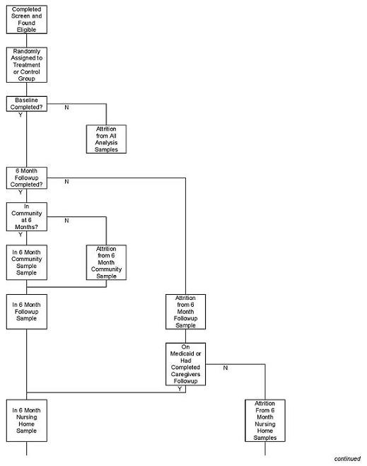
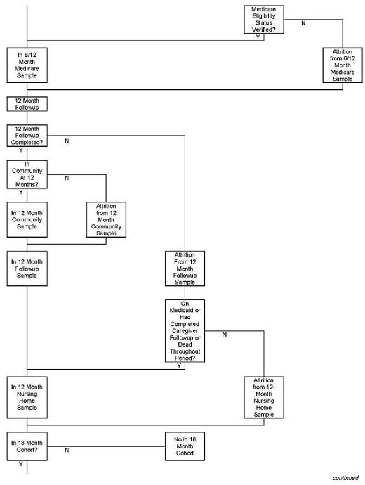
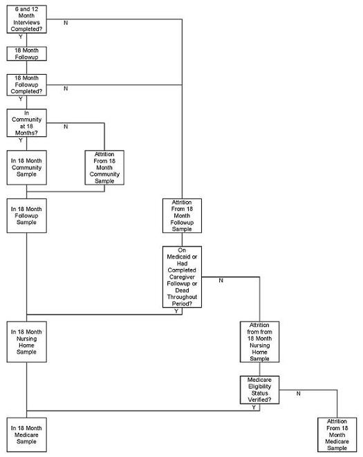
These five different sample types form a hierarchy, with each being nested, or nearly so, within the one above it.10 Figure II.1 shows the relationship between them.
Before proceeding to the examination of response rates, there are two points that should be noted. First, each of the analysis samples described above are used to examine channeling impacts on many outcome measures falling under the general area for which the samples were defined. Clearly, we cannot examine all of these estimates for evidence of attrition, so we have identified the key outcome measures within each substantive area and confined our analysis of attrition bias to these variables. The variables are listed in Chapter IV.
| FIGURE II.1: Flowchart of Inclusion In and Attrition From Analysis Samples |
|---|
 |
 |
 |
The other point to be made is that an observation can be omitted from the analysis of impacts on a given outcome measure due to item nonresponse on that variable, even if the sample member is in the appropriate analysis sample. In general, there are relatively few such cases of missing data on individual outcome variables when the observation is in the appropriate analysis sample, and, of course, which observations are missing depends on the specific variable examined. Thus, the possible effect of item nonresponse on impact estimates is ignored in this report.
B. Response Rates and Reasons for Attrition
In Table II.1, we present the full sample size and percent of the full sample included in each of the analysis samples. Figures are presented separately by model and experimental status.
The results indicate that at 6 months, 88 percent of the full sample was in the Medicare sample. Loss of observations was due almost entirely to sample members' failure to complete the baseline (as we shall see later); nonverifiability of Medicare eligibility was responsible for only about one-tenth of the cases excluded from this analysis sample.
Only 73 percent of the full sample was included in the nursing home sample, with the additional loss of observation arising because of sample member death and nonresponse to the 6 month interview. The followup sample included two thirds of the full sample, while the in-community sample at six months was comprised of the 55 percent of sample members who completed the 6 month followup and were residing in the community.
The proportions of the full sample included in the analysis samples at 12 months were comparable to those at 6 months. The proportion in the followup sample was lower, as expected, given the substantial fraction of sample members who died within the 7 to 12 month period. The proportion of the full sample included in the nursing home sample actually increased between the first and second six month periods, however, because some sample members who died within the first period were excluded from the 6 month analysis (since their utilization of-nursing homes was unknown) but included in the 12-month analysis (because their utilization was known to be zero).
Two figures are presented for the in-community sample at 12 months. The first is the proportion of the full sample that was included in this sample; the second is the proportion of those alive at the beginning of the period. The latter is the relevant measure of sample inclusion in this sample, since the in-community sample is used to estimate impacts on use of formal and informal care for sample members during the time they spent in the community. Since sample members who were deceased at the beginning of the period could never be in the community, this outcome is undefined rather than just missing for this sample. The proportion of those alive at the beginning of the 7 to 12 month period who are included in this sample is by chance the same (55 percent) as the proportion of those alive at the beginning of the 1 to 6 month period (the full sample) who are included in the 6 month in-community sample.
| TABLE II.1: Percent of Full Sample Included in Analysis Samples | |||||||||
|---|---|---|---|---|---|---|---|---|---|
| Basic Model | Financial Control Model | Full Sample | |||||||
| Treatments | Controls | Total | Treatments | Controls | Total | Treatments | Controls | Total | |
| 6 MONTH OUTCOMES | |||||||||
| Number of Observations in Full Sample | 1,779 | 1,345 | 3,124 | 1,923 | 1,279 | 3,202 | 3,702 | 2,624 | 6,326 |
| Percent of Full Sample Included in: | |||||||||
| Medicare sample | 90.4 | 82.1 | 86.8 | 93.3 | 81.9 | 88.8 | 91.9 | 82.0 | 87.8 |
| Nursing home sample | 72.0 | 67.1 | 69.9 | 80.5 | 67.3 | 75.2 | 76.4 | 67.2 | 72.6 |
| Followup sample | 66.4 | 62.0 | 64.5 | 73.1 | 59.2 | 67.5 | 69.9 | 60.6 | 66.0 |
| In-community sample | 54.8 | 51.5 | 53.3 | 62.3 | 48.9 | 56.9 | 58.7 | 50.2 | 55.2 |
| 12 MONTH OUTCOMES | |||||||||
| Percent of Full Sample Included In: | |||||||||
| Medicare sample | 90.4 | 82.1 | 86.8 | 93.3 | 81.9 | 88.8 | 91.9 | 82.0 | 87.8 |
| Nursing home sample | 76.4 | 69.5 | 73.4 | 82.0 | 68.9 | 76.8 | 79.3 | 69.2 | 75.1 |
| Followup sample | 59.1 | 52.1 | 56.1 | 63.0 | 51.4 | 58.4 | 61.2 | 51.8 | 57.3 |
| In-community sample | 47.1 | 41.0 | 44.5 | 50.7 | 40.7 | 46.7 | 49.0 | 40.9 | 45.6 |
| In-community sample as % of those alive at beginning of perioda | 56.9 (1,472) | 50.6 (1,091) | 54.2 (2,563) | 60.9 (1,600) | 48.9 (1,065) | 56.1 (2,665) | 59.0 (3,072) | 49.8 (2,156) | 55.2 (5,228) |
| 18 MONTH OUTCOMES | |||||||||
| Number of Observations in 18-Month Cohort | 922 | 697 | 1,619 | 926 | 620 | 1,546 | 1,848 | 1,317 | 3,165 |
| Percent of Full Sample Included In: | |||||||||
| Medicare sample | 89.3 | 84.9 | 87.4 | 94.1 | 80.8 | 88.8 | 91.7 | 83.0 | 88.1 |
| Nursing home sample | 69.8 | 68.1 | 69.1 | 78.8 | 64.4 | 73.0 | 74.4 | 66.4 | 71.0 |
| Followup sample | 43.8 | 40.3 | 42.3 | 50.9 | 40.2 | 46.6 | 47.4 | 40.2 | 44.4 |
| In-community sample | 33.6 | 31.3 | 32.6 | 38.8 | 31.5 | 35.8 | 36.2 | 31.4 | 34.2 |
| In-community sample as % of those alive at beginning of perioda | 46.5 (667) | 44.9 (486) | 45.8 (1,153) | 53.8 (667) | 42.5 (459) | 49.2 (1,126) | 50.1 (1,334) | 43.7 (645) | 47.5 (2,279) |
| |||||||||
For the 18 month sample the sample retention rates are similar to the rates in other periods for the Medicare and nursing home samples but considerably lower for the followup and in-community samples because of additional deaths and the requirement that sample members complete both of the earlier interviews.
Comparing treatment and control groups we see that the differences in the proportion of observations available for analysis are substantial and fairly constant (about 10 percentage points) across all periods and analysis samples. Thus, the treatment/control difference for all samples appears to be due to the differential response rates at baseline. The difference is especially pronounced for the financial control model (about 13 percentage points, compared to 6 to 8 points for most samples in the basic model).
1. Reasons for Attrition
To obtain a somewhat more detailed picture of the reasons for sample loss and how it differs across experimental groups and models, we present in Table II.2a and Table II.2b a breakdown of the total attrition from the full sample by the reason data were unavailable, for each analysis sample. The results are discussed below.
The Medicare Sample. Most of the attrition from the Medicare sample occurred at baseline--11.4 percent of the screen sample overall were excluded from the Medicare sample because they did not complete a baseline interview, while an additional 0.8 percent were dropped because Medicare entitlement could not be verified or Medicare records were not obtained. Of those who attrited at baseline, 20 percent died before the interview could be conducted, and the rest either refused to complete the interview or could not be reached. Similar attrition rates occurred in the 18-month Medicare sample.
As noted above, the overall attrition rates were substantially higher in the control group than in the treatment group, especially in the financial contol model. These higher attrition rates among control group members are attributable to their higher baseline nonresponse rates. Breakdowns of the reasons for baseline nonresponse, presented later, show that controls were much more likely than treatments to refuse to participate in the baseline interview. This higher rate of refusal for controls is due to the incentives of the treatment group to respond (completion of the baseline was a requirement to receive channeling services) and to the fact that some control members were angry about being excluded from receiving channeling services.11
| TABLE II.2a: Attrition From the 6- and 12-Month Medicare, Nursing Home, and Followup Analysis Samples as a Percent of the Full Sample | |||||
|---|---|---|---|---|---|
| Basic Model | Financial Control Model | Total | |||
| Treatment | Control | Treatment | Control | ||
| FULL SAMPLE | 1779 | 1345 | 1923 | 1279 | 6326 |
| MEDICARE SAMPLE | |||||
| Deceased prior to baseline | 2.0 | 3.3 | 1.6 | 2.5 | 2.3 |
| Other baseline nonresponse | 6.2 | 13.6 | 4.4 | 15.4 | 9.1 |
| Medicare coverage unknown | 1.3 | 1.0 | 0.7 | 0.2 | 0.8 |
| Total Attrition Rate | 9.6 | 17.9 | 6.7 | 18.1 | 12.2 |
| Observations Available for Analysis | 1608 | 1104 | 1795 | 1047 | 5554 |
| 6 MONTH NURSING HOME SAMPLE | |||||
| Attrition from Medicare sample | 9.6 | 17.9 | 6.7 | 18.1 | 12.2 |
| Died in period, no nursing home data | 9.6 | 8.1 | 7.7 | 6.0 | 8.0 |
| Alive at 6 months, no data | 8.8 | 6.8 | 5.1 | 8.5 | 7.2 |
| Total Attrition Rate | 28.0 | 32.9 | 19.5 | 32.7 | 27.4 |
| Observations Available for Analysis | 1281 | 903 | 1548 | 861 | 4593 |
| 12 MONTH NURSING HOME SAMPLE | |||||
| Attrition from Medicare sample | 9.6 | 17.9 | 6.7 | 18.1 | 12.2 |
| Died in period, no nursing home data | 6.6 | 5.8 | 6.7 | 4.8 | 6.1 |
| Alive at 12 months, no data | 7.4 | 6.8 | 4.7 | 8.2 | 6.6 |
| Total Attrition Rate | 23.6 | 30.5 | 18.0 | 31.1 | 24.9 |
| Observations Available for Analysis | 1359 | 935 | 1577 | 881 | 4752 |
| 6 MONTH FOLLOWUP SAMPLE | |||||
| Attrition at baseline | 8.2 | 16.9 | 6.0 | 17.9 | 11.0 |
| Died in period | 14.4 | 12.7 | 14.4 | 12.3 | 13.6 |
| Other followup nonresponse | 11.0 | 8.4 | 6.5 | 10.6 | 9.4 |
| Total Attrition Rate | 33.6 | 38.0 | 26.9 | 40.8 | 34.0 |
| Observations Available for Analysis | 1181 | 834 | 1405 | 757 | 4177 |
| 12 MONTH FOLLOWUP SAMPLE | |||||
| Attrition at baseline | 8.2 | 16.9 | 6.0 | 17.9 | 11.0 |
| Died before 12 month interview | 23.6 | 22.2 | 25.0 | 20.6 | 23.1 |
| Other followup nonresponse | 9.1 | 8.8 | 6.0 | 10.1 | 8.6 |
| Total Attrition Rate | 40.9 | 47.9 | 37.0 | 48.6 | 42.7 |
| Observations Available for Analysis | 1052 | 701 | 1212 | 658 | 3623 |
| TABLE II.2b: Attrition From the 18-Month Medicare, Nursing Home, and Followup Analysis Samples as a Percent of the Full Sample | |||||
|---|---|---|---|---|---|
| Basic Model | Financial Control Model | Total | |||
| Treatment | Control | Treatment | Control | ||
| 18 MONTH COHORT OF FULL SAMPLE | 922 | 697 | 926 | 620 | 3165 |
| 18 MONTH MEDICARE SAMPLE | |||||
| Deceased prior to baseline | 2.4 | 3.0 | 1.1 | 2.3 | 2.1 |
| Other baseline nonresponse | 6.6 | 11.0 | 4.1 | 16.5 | 8.8 |
| Medicare coverage unknown | 1.7 | 1.0 | 0.8 | 0.5 | 0.7 |
| Total Attrition Rate | 10.7 | 15.1 | 5.9 | 19.2 | 11.6 |
| Observations Available for Analysis | 823 | 592 | 871 | 501 | 2787 |
| 18 MONTH NURSING HOME SAMPLE | |||||
| Attrition from Medicare sample | 10.7 | 15.1 | 5.9 | 19.2 | 11.9 |
| Died in period, no nursing home data | 6.4 | 6.0 | 7.7 | 4.0 | 6.2 |
| Alive at 18 months, no data | 13.0 | 10.8 | 7.6 | 12.4 | 10.8 |
| Total Attrition Rate | 30.2 | 31.9 | 21.2 | 35.6 | 28.9 |
| Observations Available for Analysis | 644 | 475 | 730 | 399 | 2248 |
| 18 MONTH FOLLOWUP SAMPLE | |||||
| Deceased prior to baseline | 2.4 | 3.0 | 1.1 | 2.3 | 2.1 |
| Other baseline nonresponse | 6.6 | 11.0 | 4.1 | 16.5 | 8.8 |
| Deceased before scheduled 18 month interview | 30.8 | 32.3 | 34.7 | 24.8 | 31.1 |
| Nonresponse at 6 or 12 months followup | 12.4 | 10.2 | 5.6 | 12.7 | 10.0 |
| Other followup nonresponse | 4.0 | 3.2 | 3.6 | 3.5 | 3.6 |
| Total Attrition Rate | 56.2 | 59.7 | 49.1 | 59.8 | 55.6 |
| Observations Available for Analysis | 404 | 281 | 471 | 249 | 1405 |
The Nursing Home Sample. Attrition rates from these samples are relatively high, at 27 percent, 25 percent, and 29 percent for the 6-, 12-, and 18-month samples, respectively. As shown in Table II.2a and Table II.2b, the set of cases omitted from a particular nursing home sample includes all of those omitted from the Medicare sample (for the reasons given above), as well as two other groups of approximately equal size. Between 6 and 8 percent of the screen sample members were omitted from the analysis samples because they died during a period, but were not Medicaid-covered throughout the period and did not have a caregiver interview. Another 6 to 11 percent, approximately, were alive throughout a given six month period, but were excluded from the analysis sample because they did not complete the followup and did not have Medicaid coverage throughout the period.
Differences in rates of attrition from the nursing home samples by treatment status and by model exhibit patterns similar to those observed in the Medicare samples. In particular: (1) attrition rates are much higher among control group members than among treatment group members in both models; (2) control group attrition rates are similar across models; and (3) treatment group attrition rates are higher in the basic sites than in the financial control sites. When categories of attrition are considered, it becomes obvious that most of the differences between treatments and controls occurred as attrition from the Medicare samples for the reasons described above. Treatment/control differences in the remaining two categories are small, and differ little across models.
The Followup Samples. As seen in Table II.2a and Table II.2b, attrition from these samples is quite high, at about 34 percent, 43 percent, and 56 percent overall for the 6-, 12-, and 18-month samples, respectively. Sample members who failed to complete followup interviews include those who were nonrespondents at baseline (as described above and therefore ineligible for followup interviews), those who died after completing the baseline interview but before the followup interview could be attempted, and others who failed to respond to the interview because they refused to complete the interview or could not be reached. For the 6-month interview, about 11 percent of the screen sample were eliminated because they did not complete a baseline, an additional 14 percent had died by the 6-month anniversary, and about 9 percent did not respond for other reasons. Death accounts for the increasing attrition rates over time--about 23 percent died before the 12-month followup and about 31 percent of the 18-month cohort were deceased before the 18 month interview could be conducted. The proportion of the sample that dropped out for reasons other than death was fairly similar over time, although a greater proportion was excluded from the 18-month sample because of failure to complete one or both of the earlier followups.
Again, the overall attrition rates are higher for control group members than the treatment group members, and these differences are greater in the financial control model than in the basic model. Differential baseline nonresponse again accounts almost entirely for the treatment/control differences in the proportion of the samples with incomplete followups.
The In-Community Samples. Finally, rates of attrition from the in-community samples are broken down by reason, and displayed in Table II.2c. In addition to attrition due to lack of a completed followup, an additional 10 to 12 percent of the full sample were lost to analysis because the sample member was in a hospital or nursing home. This proportion of the sample who responded but were not in the community on their anniversary date was very similar across models, experimental groups, and time periods, especially for the 6 and 12 month periods.
| TABLE II.2c: Attrition From the 6, 12, and 18 Month in Community Samples as a Percent of the Full Sample | |||||
|---|---|---|---|---|---|
| Basic Model | Financial Control Model | Total | |||
| Treatment | Control | Treatment | Control | ||
| FULL SAMPLE | 922 | 697 | 926 | 620 | 6326 |
| 6-Month In-Community Sample | |||||
| Attrition at baseline | 8.2 | 16.9 | 6.0 | 17.9 | 11.0 |
| Died in period | 14.4 | 12.7 | 14.4 | 12.3 | 13.6 |
| Other followup nonresponse | 11.0 | 8.4 | 6.5 | 10.6 | 9.4 |
| Respondent not in community | 11.6 | 10.5 | 10.8 | 10.3 | 10.8 |
| Total Attrition Rate | 45.2 | 48.5 | 37.7 | 51.1 | 44.8 |
| Observations Available for Analysis | 974 | 692 | 1198 | 625 | 3489 |
| 12-Month In Community Sample | |||||
| Attrition at baseline | 8.2 | 16.9 | 6.0 | 17.9 | 11.0 |
| Died before 12 month interview | 23.6 | 22.2 | 25.0 | 20.6 | 23.1 |
| Other followup nonresponse | 9.1 | 8.8 | 6.0 | 10.1 | 8.6 |
| Respondent not in community | 12.0 | 11.1 | 12.3 | 10.7 | 11.7 |
| Total Attrition Rate | 52.9 | 59.0 | 49.3 | 59.3 | 54.4 |
| Observations Available for Analysis | 838 | 552 | 974 | 521 | 2885 |
| 18-Month Cohort of Full Sample | 922 | 697 | 926 | 620 | 3165 |
| Attrition at baseline | 9.0 | 14.0 | 5.2 | 18.8 | 11.9 |
| Deceased before scheduled 18 month interview | 30.8 | 32.3 | 34.7 | 24.8 | 31.1 |
| Nonresponse at 6 or 12 month followup | 12.4 | 10.2 | 5.6 | 12.7 | 10.0 |
| Other followup nonresponse | 4.0 | 3.2 | 3.6 | 3.5 | 3.6 |
| Respondent not in community | 10.2 | 9.0 | 12.1 | 8.7 | 9.2 |
| Total Attrition Rate | 66.4 | 68.7 | 61.2 | 68.5 | 65.8 |
| Observations Available for Analysis | 310 | 218 | 359 | 195 | 1082 |
2. Reasons for Interview Nonresponse
The previous discussion indicated that nonresponse to the interviews, especially the baseline, was the primary reason for treatment/control differences in the proportion of the full sample that was available for analysis in any area. To understand these differences in nonresponse, Table II.3 disaggregates the nonresponse category by the reasons for nonresponse, again by model and by treatment status. From this table we learn that control group members are considerably more likely than treatment group members to refuse the baseline interview in both models.12 In none of the followup interviews do we find such large treatment/control differences in reasons for nonresponse as in the baseline. As expected, death accounts for most of the nonresponse at each of the followup interviews for all groups, ranging from 12.3 percent of the sample at 6 months to 34.8 percent at 18 months.13
| TABLE II.3: Reasons for Incomplete Interviews at Baseline and at 6, 12, and 18 Month Followup (Percent of Full Sample) | ||||||
|---|---|---|---|---|---|---|
| Basic Case Management Model | Financial Control Model | |||||
| Treatment | Control | Total | Treatment | Control | Total | |
| BASELINE | ||||||
| Completed Baseline | 92.1 | 83.2 | 88.3 | 94.4 | 82.4 | 89.6 |
| Not Completed Baseline Due to: | ||||||
| Deceased prior to baseline | 2.0 | 3.3 | 2.6 | 1.6 | 2.5 | 2.0 |
| Refusal | 2.6 | 10.9 | 6.2 | 1.4 | 10.6 | 5.1 |
| Moved out of area | 0.3 | 0.1 | 0.3 | 0.2 | 0.2 | 0.2 |
| Unable to locate respondent or proxy | 0.2 | 0.4 | 0.3 | 0.2 | 0.9 | 0.4 |
| Othera | 2.8 | 1.9 | 2.4 | 2.3 | 3.4 | 2.7 |
| Total Attrition | 7.9 | 16.8 | 11.7 | 5.6 | 17.6 | 10.4 |
| Total | 100.0 | 100.0 | 100.0 | 100.0 | 100.0 | 100.0 |
| Sample Size | 1779 | 1345 | 3124 | 1923 | 1279 | 3202 |
| 6-MONTH FOLLOWUP | ||||||
| Completed Followup | 66.4 | 62.0 | 64.5 | 73.1 | 59.2 | 67.5 |
| Not Completed Baseline Due to: | ||||||
| No interview attemptedc | 7.9 | 16.8 | 11.7 | 5.6 | 17.6 | 10.4 |
| Deceasedb | 14.4 | 12.6 | 13.6 | 14.5 | 12.3 | 13.6 |
| Refusal | 5.3 | 4.1 | 4.8 | 2.1 | 5.8 | 3.6 |
| Moved out of area | 1.8 | 1.0 | 1.4 | 1.0 | 1.6 | 1.2 |
| Unable to locate respondent or proxy | 0.7 | 0.7 | 0.7 | 0.5 | 1.2 | 0.8 |
| Othera | 3.5 | 2.8 | 3.2 | 3.3 | 2.4 | 2.9 |
| Total Attrition | 33.6 | 38.0 | 35.5 | 26.9 | 40.8 | 32.5 |
| Total | 100.0 | 100.0 | 100.0 | 100.0 | 100.0 | 100.0 |
| Sample Size | 1779 | 1345 | 3124 | 1923 | 1279 | 3202 |
| 12-MONTH FOLLOWUP | ||||||
| Completed Followup | 59.1 | 52.1 | 56.1 | 63.0 | 51.4 | 58.4 |
| Not Completed Baseline Due to: | ||||||
| No interview attemptedc | 7.9 | 16.8 | 11.7 | 5.6 | 17.6 | 10.4 |
| Deceased | 23.6 | 22.2 | 23.0 | 25.0 | 20.6 | 23.2 |
| Refusal | 4.7 | 5.1 | 4.8 | 2.1 | 5.4 | 3.4 |
| Moved out of area | 2.1 | 1.3 | 1.8 | 1.7 | 1.6 | 1.7 |
| Unable to locate respondent or proxy | 0.9 | 0.9 | 0.9 | 0.3 | 1.0 | 0.6 |
| Othera | 1.6 | 1.6 | 1.6 | 2.2 | 2.3 | 2.2 |
| Total Attrition | 40.9 | 47.9 | 43.9 | 37.0 | 48.6 | 41.6 |
| Total | 100.0 | 100.0 | 100.0 | 100.0 | 100.0 | 100.0 |
| Sample Size | 1779 | 1345 | 3124 | 1923 | 1279 | 3202 |
| 18-MONTH FOLLOWUP | ||||||
| Completed Followup | 43.8 | 40.3 | 42.3 | 50.9 | 40.2 | 46.6 |
| Not Completed Baseline Due to: | ||||||
| No interview attemptedc | 21.4 | 24.2 | 22.6 | 10.8 | 31.5 | 19.1 |
| Deceased | 30.8 | 32.3 | 31.4 | 34.8 | 24.8 | 30.8 |
| Refusal | 1.2 | 0.4 | 0.9 | 0.6 | 1.6 | 1.0 |
| Moved out of area | 0.4 | 1.1 | 0.7 | 0.4 | 0.2 | 0.3 |
| Unable to locate respondent or proxy | 0.0 | 0.4 | 0.2 | 0.4 | 0.2 | 0.3 |
| Othera | 2.4 | 1.1 | 1.9 | 2.1 | 1.6 | 1.9 |
| Total Attrition | 56.2 | 59.7 | 57.7 | 49.1 | 59.8 | 53.4 |
| Total | 100.0 | 100.0 | 100.0 | 100.0 | 100.0 | 100.0 |
| Sample Sized | 922 | 697 | 1619 | 926 | 620 | 1546 |
NOTE: The source for this table is 6,326 completed screen interviews, and information gathered through followup interviews, client tracking, and contact sheets.
| ||||||
C. Treatment/Control Group Differences in Characteristics in the Analysis Samples
As explained in Section A, the experimental design of the evaluation ensured that, subject to chance variation, the treatment and control groups were initially made up of individuals with similar (measured and unmeasured) characteristics. In order to be able to interpret treatment/control differences in outcomes as valid estimates of channeling's impact, it is important to ensure that the initial similarity is not undone by the effects of attrition. In an earlier report (Brown and Harrigan, 1983) the similarity of the treatment and control groups at randomization was confirmed by using data collected at the screen to compare the characteristics of the two groups. That analysis is extended in this chapter by estimating treatment/control differences on screen characteristics for the samples available for analysis at 6, 12, and 18 months after randomization. Because there are so many analysis samples and because the treatment/control differences in the proportion of the sample with available data for any analysis appear to be driven by the treatment/control differences in interview nonresponse, we confine our investigation of initial differences to the followup samples.
Treatment/control differences in the following screen characteristics are presented in Table II.4a (basic sites) and Table II.4b (financial control sites):
- Impairments on activities of daily living; incontinence
- How referred to channeling (by hospital or nursing home, home health agency, other)
- Ethnicity (black, hispanic, white)
- Sex
- Age
- Cognitive impairment (severe, moderate, mild/none)
- Interviewer-assessed unmet needs (low, medium, high)
- Whether sample member has Medicaid coverage
- Whether a proxy completed or helped complete the'screen
- Whether regular help received with
- meal preparation
- housework or shopping
- taking medicine
- medical treatments at home
- personal care
- Income (0-500, 501-1000, over 1000 dollars per month)
- Whether on waiting list or applied for nursing home
- Number of contacts required to obtain screen interview
- Number of missing items on the screen
- Whether expect help will be needed to complete the baseline and followup interviews
- Living arrangement (with child, with spouse but not with child, with other, or alone)
Some item nonresponse occurred for the screen variables. To some extent, item nonresponse was minimized, where appropriate, by imputing the baseline value of the measurement of the same characteristic. Remaining item nonresponse was dealt with by imputing the mean of the nonmissing values if only little nonresponse existed, or including a separate nonresponse category if item nonresponse exceeded 5 percent.
The numbers of primary interest in each of these tables are the treatment/control differences, estimated by regression to control for the different distribution of treatment and control groups across sites.14 The (unadjusted) treatment group means are also given as a reference point, and can be used to obtain a profile of those who remain in the samples over time.
Some differences between treatment and control groups will occur by chance; hence, we concentrate on those for which the probability that a difference of the size observed would occur by chance is less than 5 percent. In each of the tables the first column gives treatment/control differences for the full research sample, which are comparable--except for a slightly different sample definition--to those presented in Brown and Harrigan (1983).
The overall picture presented by Table II.4a and Table II.4b is that the differences between treatment and control groups are quite small, either before or after attrition, and very few are statistically significant. In the basic sites, we note significant differences in three of the 17 variables examined--ethnicity (at 6 and 12 months), number of missing items on the screen (at 6 and 12 months), and living arrangement (at 18 months only). However, the difference in missing items on the screen existed at randomization and thus is not attributable to treatment/control differences in attrition. Continence, on the other hand, was significantly different for the two groups at randomization but not at followup. In the financial control model, however, treatment/control differences in referral source (at 18 months) and income (at 6 and 12 months) widened and became statistically significant. Thus, of the 51 comparisons presented for each model (17 variables at three points in time), only 3 in each model--about what would be expected to occur by chance--were statistically significant that were not explainable by significant differences at the time of randomization. This is about the number of such differences that might be expected to occur by chance in this number of tests.
In addition to the fact that there were few instances of statistically significant differences, the types of variables for which they were found and the lack of pattern in these results increase the belief that attrition did not lead to serious differences between the two groups. The lack of difference between the two groups on ADL, unmet needs, and other indicators of impairment increases our confidence that the two groups do not differ on unobserved dimensions of health status or other .factors that are related to outcomes of interest. The two significant differences which appear only at 18 months seem to be more happenstance than systematic differences in attrition patterns.
Overall, the pattern and magnitude of treatment/control differences on screen characteristics for the followup samples at 6, 12, and 18 months lead us to believe that attrition did not result in treatment and control groups that differ substantially on observed screen characteristics. However, this does not ensure that estimates of channeling impacts are not biased by attrition. The conditions which lead to bias is the topic of the next chapter.
| TABLE II.4a: Comparison of Screen Characteristics of Treatments and Controls in Basic Sties Who Completed 6, 12, and 18 Month Followup Interviews (Percent, unless otherwise indicated) | ||||||||||||
|---|---|---|---|---|---|---|---|---|---|---|---|---|
| Screen Characteristics | Full Screen Sample | For Sample Members Completing: | ||||||||||
| 6-Month Interview | 12-Month Interview | 18-Month Interview | ||||||||||
| Treatment Group Mean | T/C Differences | t- value | Treatment Group Mean | T/C Differences | t- value | Treatment Group Mean | T/C Differences | t- value | Treatment Group Mean | T/C Differences | t- value | |
| IMPAIRMENT OF ABILITY TO PERFORM ACTIVITIES OF DAILY LIVING (ADL) | ||||||||||||
| Extremely severe | 21.3 | -1.4 | (-0.92) | 18.0 | -2.6 | (-1.46) | 16.4 | -1.6 | (-0.85) | 18.1 | 1.3 | (0.45) |
| Highly severe | 34.9 | 0.6 | (0.35) | 35.4 | 2.2 | (1.03) | 36.0 | 3.9 | (1.66) | 34.4 | 5.8 | (1.57) |
| Moderately severe | 23.3 | -0.4 | (-0.27) | 22.9 | -2.4 | (-1.25) | 23.4 | -3.8 | (-1.82) | 22.5 | -5.2 | (-1.56) |
| Mild or none | 20.5 | 1.2 | (0.84) | 23.7 | 2.8 | (1.54) | 24.1 | 1.5 | (0.76) | 25.0 | -1.9 | (-0.58) |
| CONTINENCE | ||||||||||||
| Continent | 41.3 | 0.1 | (0.04) | 43.4 | -0.8 | (-0.34) | 44.2 | -2.4 | (-0.98) | 46.0 | -2.0 | (-0.50) |
| Incontinent | 50.5 | 2.1 | (1.18) | 50.0 | 1.9 | (0.84) | 49.5 | 2.9 | (1.21) | 47.0 | 2.1 | (0.54) |
| Colostomy bag, device, need help | 8.1 | -2.2* | (-1.98) | 6.5 | -1.1 | (-0.91) | 6.3 | -0.6 | (-0.43) | 6.9 | -0.1 | (-0.06) |
| REFERRAL SOURCE | ||||||||||||
| Hospital or nursing home | 28.5 | -1.3 | (-0.77) | 25.7 | -0.4 | (-0.18) | 26.3 | -0.4 | (-0.19) | 27.2 | 3.9 | (1.16) |
| Home health agency | 11.5 | 0.1 | (0.07) | 11.6 | -0.2 | (-0.11) | 10.6 | 0.4 | (0.26) | 6.9 | -3.0 | (-1.14) |
| Neither | 60.0 | 1.2 | (0.67) | 62.7 | 0.5 | (0.25) | 63.0 | -0.0 | (-0.02) | 65.8 | -0.9 | (0.25) |
| ETHNICITY | ||||||||||||
| Black | 21.9 | -1.8 | (-1.35) | 21.8 | -3.2* | (-1.97) | 21.0 | -4.2* | (-2.38) | 23.0 | -4.5 | (-1.60) |
| Hispanic | 1.9 | 0.1 | (0.11) | 2.4 | -0.3 | (-0.32) | 2.6 | -0.4 | (-0.45) | 3.0 | -0.5 | (-0.32) |
| White | 76.2 | 1.7 | (1.22) | 75.9 | 3.5* | (1.99) | 76.4 | 4.6* | (2.43) | 74.0 | 5.0 | (1.66) |
| SEX | ||||||||||||
| Male | 28.6 | -0.0 | (-0.01) | 25.0 | -0.4 | (-0.19) | 23.5 | 0.6 | (0.30) | 22.0 | -0.6 | (-0.18) |
| AGE (in years) | 79.1 | 0.1 | (0.48) | 78.9 | 0.1 | (0.34) | 78.9 | 0.3 | (0.88) | 78.9 | 0.8 | (1.35) |
| COGNITIVE IMPAIRMENT | ||||||||||||
| Severe | 14.8 | -0.5 | (-0.35) | 13.6 | -1.0 | (-0.63) | 14.0 | -0.2 | (-0.09) | 14.6 | -1.3 | (-0.46) |
| Moderate | 27.5 | 1.0 | (0.62) | 25.8 | 1.1 | (0.50) | 24.3 | 0.6 | (0.29) | 25.2 | 4.3 | (1.24) |
| Mild | 49.2 | 0.1 | (0.05) | 50.8 | 1.0 | (0.45) | 51.8 | 1.2 | (0.50) | 48.8 | -0.5 | (-0.13) |
| (Missing) | 8.5 | -0.7 | (-0.91) | 9.7 | -1.0 | (-1.07) | 10.0 | -1.7 | (-1.56) | 11.4 | -2.6 | (-1.40) |
| INTERVIEWER ASSESSED UNMET NEEDS | ||||||||||||
| Low | 29.6 | -2.9 | (-1.80) | 29.6 | -1.6 | (-0.78) | 29.8 | 0.9 | (0.40) | 30.7 | 0.5 | (0.13) |
| Medium | 33.0 | 1.6 | (0.93) | 31.2 | -2.3 | (-1.07) | 31.7 | -3.2 | (-1.40) | 26.5 | -0.9 | (-0.24) |
| High | 33.1 | 0.2 | (0.14) | 34.8 | 2.9 | (1.44) | 34.4 | 1.5 | (0.69) | 38.4 | 0.4 | (-0.12) |
| (Missing) | 4.4 | 1.1 | (1.32) | 4.3 | 0.9 | (0.93) | 4.1 | 0.9 | (0.80) | 4.5 | 0.8 | (0.47) |
| MEDICAID INSURANCE | 20.6 | 0.1 | (0.23) | 21.2 | -1.6 | (-0.83) | 20.8 | -2.1 | (-1.01) | 20.8 | -2.0 | (-0.57) |
| PROXY USE AT SCREEN | 65.7 | -0.4 | (-0.23) | 61.8 | -0.7 | (-0.33) | 61.2 | 1.3 | (0.58) | 59.2 | 2.1 | (0.57) |
| REGULAR HELP RECEIVED WITH: | ||||||||||||
| Meal preparation | 74.4 | -1.6 | (-1.18) | 71.3 | -2.9 | (-1.61) | 70.7 | -1.9 | (-0.94) | 70.3 | -3.4 | (-1.05) |
| Housework, shopping | 78.2 | -1.0 | (-0.81) | 76.0 | -2.6 | (-1.56) | 75.2 | -2.2 | (-1.23) | 75.3 | -1.7 | (-0.58) |
| Taking medicine | 56.4 | -1.5 | (-0.92) | 53.0 | -0.9 | (-0.41) | 52.3 | 0.6 | (0.26) | 52.1 | 1.2 | (0.34) |
| Medical treatments at home | 43.5 | 0.0 | (0.00) | 40.3 | -0.5 | (-0.23) | 39.1 | -1.7 | (-0.70) | 37.4 | 0.4 | (0.11) |
| Personal care | 68.9 | -1.2 | (-0.77) | 65.2 | -1.8 | (-0.94) | 64.3 | -0.3 | (-0.12) | 62.7 | 2.3 | (0.70) |
| INCOME | ||||||||||||
| <$500/mo. | 57.7 | -1.3 | (-0.76) | 60.3 | -1.6 | (-0.75) | 60.3 | -2.7 | (-1.13) | 64.4 | 3.0 | (0.82) |
| $500-$999/mo. | 33.8 | -0.0 | (-0.02) | 31.8 | -0.0 | (-0.01) | 31.9 | 0.8 | (0.34) | 27.7 | -2.6 | (-0.74) |
| >$1000/mo. | 8.5 | 1.4 | (1.45) | 8.0 | 1.7 | (1.45) | 7.8 | 1.9 | (1.54) | 7.9 | -0.4 | (-0.21) |
| ON WAITING LIST (or applied for) NURSING HOME | 11.3 | 0.7 | (0.66) | 9.7 | -0.7 | (-0.58) | 10.0 | -0.2 | (-0.15) | 11.4 | 0.2 | (0.09) |
| NUMBER OF CONTACTS TO OBTAIN SCREEN INTERVIEWS | 2.2 | 0.0 | (0.81) | 2.1 | 0.0 | (0.50) | 2.1 | 0.1 | (1.04) | 2.2 | 0.1 | (0.85) |
| NUMBER OF MISSING ITEMS ON SCREEN | 0.8 | -0.2* | (-2.52) | 0.9 | -0.2* | (-2.12) | 0.9 | -0.2* | (-2.10) | 1.0 | -0.0 | (-0.02) |
| NEEDED HELP TO COMPLETE BASELINE | 54.1 | -0.5 | (-0.28) | 50.9 | -0.8 | (-0.38) | 49.4 | -0.5 | (-0.20) | 47.4 | -2.7 | (-0.71) |
| LIVING ARRANGEMENT | ||||||||||||
| With child | 22.9 | -1.3 | (-0.88) | 22.8 | -0.7 | (-0.40) | 22.1 | 0.1 | (0.03) | 21.5 | 3.2 | (1.03) |
| With spouse, not with child | 28.7 | 2.3 | (1.40) | 28.5 | 2.7 | (1.34) | 27.8 | 4.0 | (1.86) | 28.7 | 2.7 | (0.78) |
| With other (no spouse or child) | 9.4 | -0.4 | (-0.41) | 8.5 | -1.3 | (-1.04) | 8.5 | -1.7 | (-1.27) | 8.7 | -4.7* | (-2.14) |
| Alone | 35.8 | -0.7 | (-0.42) | 36.7 | -1.0 | (-0.46) | 38.2 | -3.1 | (-1.28) | 35.9 | -4.1 | (-1.07) |
| (Missing) | 3.2 | 0.2 | (0.26) | 3.5 | 0.3 | (0.44) | 3.5 | 0.7 | (0.78) | 5.2 | 2.8* | (2.19) |
| MAXIMUM SAMPLE SIZE | (N=3124) | (N=2015) | (N=1753) | (N=685) | ||||||||
| NOTE: Treatment/control (T/C) differences were estimated controlling for site. Treatment group means are unadjusted means, provided as a reference. * Statistically significant at the 5 percent level for a two-tailed test. ** Statistically significant at the 1 percent level for a two-tailed test. | ||||||||||||
| TABLE II.4b: Comparison of Screen Characteristics of Treatments and Controls in Financial Control Sites Who Completed 6, 12, and 18 Month Followup Interviews (Percent, unless otherwise indicated) | ||||||||||||
|---|---|---|---|---|---|---|---|---|---|---|---|---|
| Screen Characteristics | Full Screen Sample | For Sample Members Completing: | ||||||||||
| 6-Month Interview | 12-Month Interview | 18-Month Interview | ||||||||||
| Treatment Group Mean | T/C Differences | t- value | Treatment Group Mean | T/C Differences | t- value | Treatment Group Mean | T/C Differences | t- value | Treatment Group Mean | T/C Differences | t- value | |
| IMPAIRMENT OF ABILITY TO PERFORM ACTIVITIES OF DAILY LIVING (ADL) | ||||||||||||
| Extremely severe | 26.4 | -0.0 | (-0.03) | 23.8 | 1.2 | (0.65) | 21.8 | 0.6 | (0.30) | 20.4 | -2.0 | (-0.66) |
| Highly severe | 35.2 | 0.7 | (0.43) | 35.2 | 1.6 | (0.73) | 36.1 | 2.5 | (1.05) | 36.7 | 5.9 | (1.59) |
| Moderately severe | 20.4 | -1.2 | (-0.80) | 21.8 | -3.4 | (-1.78) | 22.4 | -2.3 | (-1.09) | 24.2 | 1.3 | (0.38) |
| Mild or none | 18.0 | 0.5 | (0.35) | 19.1 | 0.7 | (0.38) | 19.7 | -0.7 | (-0.36) | 18.7 | -5.2 | (-1.59) |
| CONTINENCE | ||||||||||||
| Continent | 42.7 | 0.6 | (0.31) | 44.6 | 0.6 | (0.27) | 47.4 | 2.3 | (0.92) | 48.6 | 6.1 | (1.54) |
| Incontinent | 45.2 | -0.2 | (-0.14) | 45.7 | -1.2 | (-0.53) | 43.5 | -2.9 | (-1.20) | 42.3 | -6.2 | (-1.57) |
| Colostomy bag, device, need help | 12.1 | -0.3 | (-0.28) | 9.7 | 0.6 | (0.46) | 9.2 | 0.7 | (0.52) | 9.1 | 0.1 | (0.04) |
| REFERRAL SOURCE | ||||||||||||
| Hospital or nursing home | 32.2 | -0.9 | (-0.52) | 28.9 | 1.2 | (0.61) | 28.4 | 1.6 | (0.75) | 28.9 | 6.4 | (1.86) |
| Home health agency | 21.5 | -1.2 | (-0.94) | 21.8 | 0.7 | (-0.40) | 21.1 | -1.8 | (-1.00) | 20.0 | -6.9** | (-2.59) |
| Neither | 46.3 | 2.1 | (1.20) | 49.3 | -0.6 | (-0.26) | 50.5 | 0.1 | (0.06) | 51.2 | -0.5 | (0.14) |
| ETHNICITY | ||||||||||||
| Black | 23.3 | -1.0 | (-0.77) | 22.9 | -2.3 | (-1.41) | 22.1 | -2.4 | (-1.35) | 19.3 | -3.7 | (-1.29) |
| Hispanic | 5.2 | -0.0 | (-0.08) | 5.7 | -1.1 | (-1.31) | 5.9 | -0.6 | (-0.69) | 7.9 | -0.5 | (-0.29) |
| White | 71.5 | 1.1 | (0.76) | 71.4 | 3.4 | (1.94) | 71.9 | 3.0 | (1.59) | 72.8 | 4.1 | (1.35) |
| SEX | ||||||||||||
| Male | 29.2 | 1.6 | (0.99) | 26.5 | 0.4 | (0.22) | 25.3 | 1.0 | (0.48) | 24.6 | 2.0 | (0.61) |
| AGE (in years) | 80.1 | 0.3 | (1.08) | 80.0 | 0.5 | (1.32) | 79.7 | 0.2 | (0.50) | 78.9 | -0.6 | (-1.09) |
| COGNITIVE IMPAIRMENT | ||||||||||||
| Severe | 17.1 | 1.6 | (1.19) | 16.6 | 1.7 | (1.04) | 16.6 | 1.4 | (0.79) | 17.4 | 3.7 | (1.28) |
| Moderate | 36.0 | -0.9 | (-0.53) | 35.7 | 0.9 | (0.42) | 35.4 | 2.9 | (1.28) | 33.8 | 1.3 | (0.37) |
| Mild | 44.5 | -0.7 | (-0.41) | 44.8 | -2.6 | (-1.14) | 45.0 | -4.2 | (-1.73) | 45.0 | -3.8 | (-0.98) |
| (Missing) | 2.5 | 0.0 | (0.05) | 2.9 | -0.0 | (-0.03) | 3.1 | -0.1 | (-0.05) | 3.8 | -1.1 | (-0.62) |
| INTERVIEWER ASSESSED UNMET NEEDS | ||||||||||||
| Low | 29.8 | -1.3 | (-0.78) | 30.0 | -1.9 | (-0.94) | 28.9 | -2.5 | (-1.17) | 29.7 | -5.1 | (-1.45) |
| Medium | 34.9 | 0.9 | (0.52) | 36.5 | 2.8 | (1.32) | 37.5 | 4.1 | (1.74) | 41.2 | 4.8 | (1.31) |
| High | 28.4 | 0.6 | (0.37) | 26.9 | -0.3 | (-0.15) | 27.0 | -0.5 | (-0.24) | 22.9 | 1.4 | (0.40) |
| (Missing) | 6.9 | -0.2 | (-0.27) | 6.5 | -0.6 | (-0.63) | 6.6 | -1.0 | (-0.91) | 6.2 | -1.1 | (-0.64) |
| MEDICAID INSURANCE | 23.4 | -0.7 | (-0.47) | 23.9 | -3.5 | (-1.85) | 24.6 | -3.6 | (-1.72) | 33.3 | -3.9 | (1.11) |
| PROXY USE AT SCREEN | 68.1 | -0.9 | (-0.53) | 66.6 | -0.5 | (-0.22) | 65.3 | -1.0 | (-0.91) | 61.8 | -1.8 | (-0.48) |
| REGULAR HELP RECEIVED WITH: | ||||||||||||
| Meal preparation | 80.5 | -1.9 | (-1.34) | 79.0 | -1.7 | (-0.91) | 78.7 | -0.1 | (-0.03) | 76.4 | 2.1 | (0.64) |
| Housework, shopping | 82.7 | -1.3 | (-1.02) | 82.3 | -0.5 | (-0.28) | 81.5 | -0.9 | (-0.49) | 79.7 | -1.2 | (-0.43) |
| Taking medicine | 64.9 | -1.5 | (-0.90) | 61.7 | -1.1 | (-0.49) | 61.2 | 0.7 | (0.32) | 57.7 | 1.8 | (0.49) |
| Medical treatments at home | 54.5 | -1.4 | (-0.81) | 51.0 | 0.5 | (0.24) | 49.8 | -0.6 | (-0.24) | 48.5 | 4.2 | (1.10) |
| Personal care | 77.7 | -2.4 | (-1.63) | 76.1 | -1.8 | (-0.95) | 75.3 | -2.2 | (-1.04) | 72.2 | -3.5 | (-1.04) |
| INCOME | ||||||||||||
| <$500/mo. | 58.0 | -1.5 | (-0.86) | 57.9 | -3.4 | (-1.55) | 58.4 | -3.9 | (-1.64) | 62.8 | -1.6 | (-0.43) |
| $500-$999/mo. | 36.0 | 2.6 | (1.51) | 36.2 | 4.6* | (2.17) | 35.6 | 4.9* | (2.15) | 31.2 | 0.8 | (0.22) |
| >$1000/mo. | 6.0 | -1.1 | (-1.14) | 5.9 | -1.2 | (-1.04) | 5.9 | -1.0 | (-0.85) | 5.9 | 0.9 | (0.43) |
| ON WAITING LIST (or applied for) NURSING HOME | 8.1 | -1.2 | (-1.15) | 7.6 | -0.5 | (-0.42) | 7.8 | -0.3 | (-0.24) | 7.9 | 0.3 | (0.14) |
| NUMBER OF CONTACTS TO OBTAIN SCREEN INTERVIEWS | 2.4 | 0.0 | (0.73) | 2.4 | 0.0 | (0.14) | 2.4 | 0.1 | (1.29) | 2.4 | 0.1 | (0.75) |
| NUMBER OF MISSING ITEMS ON SCREEN | 1.3 | -0.2* | (-2.04) | 1.3 | -0.1 | (-1.33) | 1.4 | -0.2 | (-1.90) | 1.3 | -0.0 | (-0.03) |
| NEEDED HELP TO COMPLETE BASELINE | 56.5 | -1.6 | (-0.89) | 56.1 | -1.3 | (-0.59) | 54.9 | -0.5 | (-0.19) | 54.7 | 4.3 | (1.11) |
| LIVING ARRANGEMENT | ||||||||||||
| With child | 21.2 | -0.2 | (-0.13) | 20.8 | -1.3 | (-0.72) | 20.0 | -1.2 | (-0.62) | 18.7 | -1.3 | (-0.42) |
| With spouse, not with child | 29.1 | 0.8 | (0.47) | 28.0 | 0.2 | (0.10) | 28.2 | 2.3 | (1.04) | 29.7 | 0.1 | (0.03) |
| With other (no spouse or child) | 7.6 | 0.1 | (0.09) | 8.0 | 0.6 | (0.49) | 7.6 | 0.8 | (0.57) | 6.8 | -0.9 | (-0.43) |
| Alone | 38.9 | -0.9 | (-0.50) | 40.3 | -0.1 | (-0.04) | 41.1 | -1.9 | (-0.78) | 43.3 | 2.9 | (0.75) |
| (Missing) | 3.2 | 0.2 | (0.36) | 2.9 | 0.6 | (0.78) | 3.1 | 0.1 | (0.09) | 1.5 | -0.8 | (-0.60) |
| MAXIMUM SAMPLE SIZE | (N=3202) | (N=2162) | (N=1870) | (N=720) | ||||||||
| NOTE: Treatment/control (T/C) differences were estimated controlling for site. Treatment group means are unadjusted means, provided as a reference. * Statistically significant at the 5 percent level for a two-tailed test. ** Statistically significant at the 1 percent level for a two-tailed test. | ||||||||||||
III. HOW ATTRITION CAN LEAD TO BIAS AND A STATISTICAL PROCEDURE FOR ELIMINATING THE BIAS
In the previous chapter we found that attrition produced no systematic pattern of treatment/control differences in the observed, initial characteristics of the samples available for analysis. This finding does not rule out the possibility that at the time of follow up the two groups differ on unmeasured characteristics that also affect the level of a particular outcome measure. If, as a consequence of attrition, the treatment and control groups differ on average on these unmeasured characteristics, then impact estimates that do not control for these differences will be biased.
In this chapter we outline, first informally and later using statistical notation, the conditions under which attrition bias may arise. Next, we outline a statistical procedure, due to Heckman (1976, 1979) that corrects for possible bias. Finally, we show how the direction of the bias can be determined when some prior knowledge exists concerning the mechanism causing attrition.
We focus here on giving a heuristic explanation of the procedures. More complete coverage of statistical details and derivations of these methods and their justification is given in the references listed at the end of this report.
A. How Attrition Bias Occurs
As indicated in the previous chapter, differences between treatment and control groups on screen characteristics that arise because of different patterns of attrition do not necessarily imply that estimates of channeling impacts are biased. If nonresponse was affected only by screen characteristics (e.g., ADL), then inclusion of these screen characteristics as explanatory (auxiliary control) variables in the outcome regression would control for the effects of attrition. This fact is not widely understood. Two conditions are necessary for impact estimates to be biased: (1) attrition is affected by the outcome measure being examined (e.g., whether in a nursing home), or by some unobserved factor (e.g., health status at the time of the attempted followup) that affects both attrition and the outcome measure, and (2) the pattern of attrition differs for treatment and control groups. Thus, finding attrition-induced differences between treatment and control groups on observed characteristics would have implied two things. First, impacts would have to be estimated by regression controlling for all initial characteristics on which treatments and controls differ as a consequence of attrition. Second, attrition-induced differences on observed characteristics would raise the suspicion that treatments and controls differ on unmeasured characteristics as well.
To see how different attrition patterns affect impact estimates, consider the following example. Suppose that in the full sample, 20 percent of the treatment group and 30 percent of the control group are in a nursing home at the 6-month followup. Thus, channeling reduced the probability of being in a nursing home by 10 percentage points. However, contrast the effects on these results under two different assumptions about the mechanism governing attrition. In the first case, assume that attrition was random within each experimental group--that is, attrition was affected only by experimental status: controls have a 70 percent probability of response and treatments have an 80 percent probability. Clearly, restricting the analysis to just the responders would have no effect on the impact estimate: since all treatment group members have the same probability of response, the proportion of responders in nursing homes is the same as the proportion for the full sample (20 percent), and similarly 30 percent of the controls who respond to the interview will be in nursing homes. Hence, the impact estimate of 10 percentage points is unaffected by attrition, even though the attrition rates are different for treatments and controls. Furthermore, although we do not show this here, the same results hold if attrition is affected by any screen characteristic that is controlled for.
Consider how our conclusions about the effects of attrition change, however, if the probability of response is also affected by the value of the outcome being examined. For example, suppose that the probability of response among those who are in a nursing home at followup (Y=I) is only 50 percent for treatment group members and 40 percent for control group members. Suppose that the probabilities of response for those not in nursing homes (Y=0) are 95 percent for the treatment group and 85 percent for the control group (i.e., for each value of Y, treatment group members are 10 percentage points more likely to respond than controls). In this case, the treatment and control group means for the responders only (R=1) are:15
| Treatment group: | Estimated proportion in nursing homes for responders | = | responders in nursing homes |
|---|---|---|---|
| (responders in nursing homes + responders not in nursing homes) | |||
| = | 0.20 * 0.50 * N / (0.20 * 0.50 + 0.80 * 0.95) * N | ||
| = | 11.6% | ||
| Control group: | Estimated proportion in nursing homes | = | 0.30 * 0.40 * N / (0.30 * 0.40 + 0.70 * 0.84) * N |
| = | 16.8% | ||
Note that the proportion of responders in nursing homes is much smaller than the values that would have been obtained if no attrition occurred (about half as large). More important, however, we see that subtracting the control group mean from the treatment group mean for respondents gives a predicted impact of channeling on nursing home placement of -5.2 percentage points, about half the true impact in this example.
These overly simplified examples demonstrate how different mechanisms of attrition may or may not cause bias in impact estimates. Overall attrition rates for treatment and control groups in the second example are 14 and 28.5 percent, respectively--quite close to the rates actually observed for some of our analysis samples. An attrition mechanism of this type could result in estimated impacts that are too small to be statistically significant, for cases in which the estimate for the full sample would have been large and highly significant.
The statistical correction procedure described in this chapter controls for attrition by determining whether responding sample members who have a relatively low predicted probability of remaining in the sample (given their screen characteristics) are more likely to have a larger (or smaller) than expected value of the outcome (Y), given the values of auxiliary control variables. This is determined by obtaining for each observation a predicted "attrition-correction" term and including it in the regression equation used to estimate channeling impacts. If this type of correlation between unobserved factors in the attrition equation and unobserved factors in the outcome equation does exist: the coefficient on the correction term will have a significant coefficient. If, in addition, attrition is affected by experimental status, the estimated channeling impact will change substantially. The statistical procedure is described below.
B. A Joint Model of Impacts and Attrition
Regression analysis was used throughout the evaluation of channeling impacts to eliminate potential bias in impact estimates that could arise due to treatment/control differences on observed characteristics at baseline, to control for the different distribution of treatment and control groups across sites, and to provide more efficient impact estimates than a simple treatment/control group comparison of means would yield. The regression model used to estimate channeling's impacts can be described as follows. Let Y1 be the outcome of interest, such as number of hospital days or number of nursing home days. Define TB = 1 if the sample member belongs to the treatment group in the basic case management model, and TB = 0 if he or she does not. Similarly, define TF = 1 if the sample member belongs to the treatment group in the financial control model, and TF = 0 otherwise. Finally, define a set of auxiliary control variables (X1) such as site, sex, race, income, and impairment in functioning. These variables are included in the outcome equation to control for preexisting differences between sample members on characteristics that affect the value of the outcome. The model is then
| (1) | Y1 | = | aBTB + aFTF + X1b1 + u1 |
|---|---|---|---|
| = | Zb = u1 |
where aB and aF are the estimates of the impact of channeling on the .outcome, Y1, for the basic and financial control models, respectively; b1 is a vector of coefficients on the auxiliary variables; and u1 is the disturbance term capturing all of the unobserved factors which influence Y1. To facilitate the exposition below, this equation is rewritten in terms of Z and b, where Z is a vector that contains variables TB, TF, and X1, and b is the true, unobserved value of the regression parameters (aB, aF, and b1) in equation (1). In the absence of sample attrition, if the random assignment to treatment or control groups was performed correctly and the usual assumptions of least-squares regression are satisfied,16 then regression estimates of aB and aF are unbiased estimates of the impacts of channeling on outcome Y1 for the basic case management and the financial control models, respectively.
As noted above, however, we are not able to estimate this model on the full sample because of attrition. To the extent that the included auxiliary control variables (X1) account fully for the effect of any differences between responders and nonresponders on the outcome variable (Y1), the estimated coefficients in equation (1), including aB and aF, remain unbiased. However, if there are unmeasured characteristics that affect both the probability of attrition and the outcome of interest, the estimated coefficients in equation (1) will in general be biased.
The following exposition describes the mechanism by which this bias occurs. Suppose that the attrition process can be described by the equations:
| (2) | Y2* | = | X2b2 + u2, and |
|---|
| (3) | Y2 | = | 1 if Y2* > 0 (in the analysis sample) |
|---|---|---|---|
| 0 if *Y2 < 0 (lost from sample due to attrition). |
The dependent variable in equation (2) is an unobserved continuous variable, Y2*, representing the sample member's propensity to respond to the interviews (or otherwise be included in a particular analysis sample). Each sample member has his or her own tendency to cooperate with the research and refuses when the perceived effort to respond exceeds a tolerance. This tendency to respond is not observed directly, but individuals with values exceeding a constant--without loss of generality assumed to be zero--are observed to respond (Y2 = 1), while those with values less than or equal to zero are nonresponders (Y2 = 0). Propensity to respond is assumed to be a function of observable characteristics, X2 (which includes treatment status and may include other variables also included in X1), as well as unobservable characteristics and circumstances, represented by the disturbance term u2, assumed to follow a standard normal distribution.17
Bias arises in the estimates of aB and aF if the unobserved factors affecting attrition (u2) are correlated with the unobserved factors (u1) that affect the outcome measure (Y1). This can be seen by examining the general expression for the vector of regression coefficients for equation (1), which we will refer to as b~:
| (4) | b~ | = | (Z ' Z) -1Z ' Y1, |
|---|---|---|---|
| = | b + (Z ' Z) -1Z ' u1. |
Without sample attrition, the expected value of the estimated regression coefficients is the true value of the parameters (b), because the last term in the expression above has an expected value of zero. With attrition, however, the expected value of b~, given that it is estimated on only observations in the analysis sample is:
| (5) | E(b~ | in the analysis sample) | ||
|---|---|---|---|
| = | b + E [(Z ' Z) Z ' u1 | Y2 = 1] | ||
| = | b + E [(Z ' Z) -1Z u1 | Y2* > 0] | ||
| = | b + E [(Z ' Z) -1Z u1 | u2 > -X2b2] | ||
| = | b + (Z ' Z) -1Z E [u1 | -X2b2]. | ||
If u1 and u2 are correlated (i.e., if there are unobserved factors that affect both Y1, and the probability of attrition), the expected value of the final expression in square brackets will not be zero, and therefore the expected value of the regression estimates of the parameters of equation (1), including the expected value of the estimates of aB and aF, will not be equal to the true values of these parameters. Thus, the estimates are biased by sample attrition, and the size and direction of the bias are unknown.18
The nature of this bias and a procedure for correcting it were expounded by Heckman (1976, 1979). Heckman showed that the bias due to sample attrition is analogous to the bias due to omitting an important explanatory variable. That is, we have
| (6) | E(Y1 | Y2* > 0) | = | Zb + E(u1 | Y2* > 0) |
|---|---|---|---|
| = | Zb + E(u1 | u2 > -X2b2). |
As noted above, one of the assumptions of least squares regression is that the expected value of u1 is zero, so estimates of b will be unbiased. However, when sample attrition exists, the regression can be estimated only on those sample members with complete data, so unbiasedness of the resulting estimates requires that the expected value of u1, conditional upon the sample members' availability for analysis, be equal to zero. If u1 and u2 are correlated, however, this conditional expectation of u1 is not zero but is a function of u2 and X2. In this case, if Y1 is regressed on Z, and there is correlation between the variables in Z and those in X2, regression estimates of b will be biased because an "omitted" term (the nonzero conditional expected value of u1) is correlated with the regressors Z. The estimated coefficients on the variables in Z, including those on treatment status, will reflect not only the effect of Z on Y1, but also the relationship between Z and the conditional expectation of u1.
In this evaluation attrition could lead to bias in estimates of channeling impacts because those conditions that lead to bias may well be present. For example, suppose that the sample members who are the most impaired at followup are least likely to respond and also likely to have systematically higher (or lower) values of Y1 (e.g., hospital days). Since the auxiliary control variables measured at screen or baseline do not fully reflect impairment levels at the time of followup, u1 and u2 will be correlated. Furthermore, many of the variables Z and X2 that affect the outcome and the likelihood of attrition, respectively, are likely to be the same or to be highly correlated (e.g., both the outcome and likelihood of attrition may be affected by treatment/control status). Thus, there is a strong possibility that the two conditions that together produce biased estimates of regression parameters may be present and, therefore, that estimates of channeling impacts will be biased by attrition.
Fortunately, with an additional assumption, a statistical correction for attrition bias is possible. Heckman showed that although the second term on the right-hand side of equation (6) is unobserved, the n term has a relatively simple form if u1 and u2 are assumed to have a bivariate normal distribution, and this term can be estimated. Heckman shows that
| (7) | E(u1 | u2 > -X2b2 | = | f(X2b2 / | |||
|---|---|---|---|---|---|---|
| F(X2b2 / | ||||||
| = | ( | |||||
where ![]() 12 is the covariance of u1 and u2,
12 is the covariance of u1 and u2, ![]() 2 is the standard deviation of u2, b2 is the vector of the estimated coefficients from the attrition equation, f(X2b2 /
2 is the standard deviation of u2, b2 is the vector of the estimated coefficients from the attrition equation, f(X2b2 / ![]() 2) is the standard normal density function evaluated at X2b2 /
2) is the standard normal density function evaluated at X2b2 / ![]() 2, and F(X2b2 /
2, and F(X2b2 / ![]() 2) is the standard normal distribution function evaluated at the same point. If the parameters b2 of the attrition equation were known, the term M could be constructed for each sample member and used as an additional variable in the regression model. Inclusion of this variable in this regression eliminates it from the error term and therefore eliminates the correlation between Z and the error term in equation (6), thereby eliminating the (asymptotic) attrition bias in estimates of b. The regression coefficient obtained on this M term is an estimate of
2) is the standard normal distribution function evaluated at the same point. If the parameters b2 of the attrition equation were known, the term M could be constructed for each sample member and used as an additional variable in the regression model. Inclusion of this variable in this regression eliminates it from the error term and therefore eliminates the correlation between Z and the error term in equation (6), thereby eliminating the (asymptotic) attrition bias in estimates of b. The regression coefficient obtained on this M term is an estimate of ![]() 12 /
12 / ![]() 2, the (normalized) covariance between u1 and u2.
2, the (normalized) covariance between u1 and u2.
The parameters b2 are not known, but can be readily estimated. Thus, the procedure developed by Heckman and used in this report to eliminate attrition bias can be described as follows:
-
Using all observations (both responders and nonresponders), estimate the parameters of the attrition model given in equations (2) and (3) using maximum likelihood probit.19
-
From the estimated probit coefficients (b2) and the data on X2, form the correction term (M) for the observations which have valid data for the outcome regression--this excludes those lost due to attrition--and estimate equation (8) by least squares:20
| (8) | Y1 | = | aBTB + aFTF + X1b1 + cM = u1*, |
|---|
where this equation is simply equation (1) with the nonzero conditional expectation (cM) of the old disturbance term plus a new disturbance term (u1*) substituted for the old disturbance term (u1). The statistical significance of c, the coefficient on M, is an indication of whether there are unobserved factors affecting both attrition and Y1, a necessary condition for the estimates of aB and aF to be biased.
In the discussion of results in the next section, we assess the extent of attrition bias in estimates of channeling impacts in two ways: first, by examining the estimate of c, to determine whether the condition necessary for bias is met, and if so, the size and sign of the correlation between the two disturbance terms; and second, by comparing the regression estimates of aB and aF obtained when potential attrition bias is not controlled for (i.e., from estimating equation (1)) to the impact estimates obtained when this potential bias is controlled for (by estimating equation (8)). In interpreting these results, it is useful to bear in mind the determinants of the bias in a particular coefficient. Inserting the expression in equation (7) into equation (5), the bias in the uncorrected estimates of aB, aF, and b1 is shown to be
| (9) | bias ≡ E(b~)-b | = | ( |
|---|---|---|---|
| = | ( |
where the term PZ,M is a vector of auxiliary regression coefficients obtained from regressing the constructed M term on the other variables (Z's) in equation (8).21 Thus, the bias in the regression coefficient on any particular explanatory variable (e.g., aB, the coefficient on TB in the outcome equation) is equal to the covariance between u1 and u2 (normalized by ![]() 2), multiplied by the coefficient on this same variable (e.g., TB) from a second, auxiliary regression of the constructed M variable on all of the Z variables.
2), multiplied by the coefficient on this same variable (e.g., TB) from a second, auxiliary regression of the constructed M variable on all of the Z variables.
The usefulness of this expression is best demonstrated by elaborating on our previous example. Suppose that we are interested in estimating the impacts of channeling on the number of hospital days (using a followup sample). Also, suppose that those who are most impaired at the time of the followup are less likely to be available for analysis than are less impaired sample members and that the effects of this impairment on hospital days is imperfectly controlled for with the baseline control variables. Since the most impaired individuals are most likely to be in a hospital and least likely to be in the analysis sample, the covariance between u1 and u2 (![]() 12) will be negative. Furthermore, since treatment group members are more likely to be available for analysis than control group members, it can be shown that the auxiliary regression coefficient of treatment status contained in PZ,M is expected to be negative.22 Thus, we would expect the attrition bias in the estimate of aB to be positive. That is, the estimated impact will be a larger number than it should be. Thus, we could find an estimated impact of zero when in fact the impact was negative, implying a reduction in hospital days due to channeling. This analytic assessment of the direction of bias is consistent with the heuristic argument that the sample members most likely to be lost to analysis are control group members with relatively large numbers of hospital days, and if these cases were appropriately represented in the analysis sample, the treatment/control difference in expected hospital days would have been a larger negative number. Based on this reasoning, the following reference table can be used to draw inferences about the expected direction of the bias (if any) due to attrition in estimates of channeling impacts:
12) will be negative. Furthermore, since treatment group members are more likely to be available for analysis than control group members, it can be shown that the auxiliary regression coefficient of treatment status contained in PZ,M is expected to be negative.22 Thus, we would expect the attrition bias in the estimate of aB to be positive. That is, the estimated impact will be a larger number than it should be. Thus, we could find an estimated impact of zero when in fact the impact was negative, implying a reduction in hospital days due to channeling. This analytic assessment of the direction of bias is consistent with the heuristic argument that the sample members most likely to be lost to analysis are control group members with relatively large numbers of hospital days, and if these cases were appropriately represented in the analysis sample, the treatment/control difference in expected hospital days would have been a larger negative number. Based on this reasoning, the following reference table can be used to draw inferences about the expected direction of the bias (if any) due to attrition in estimates of channeling impacts:
| Expected Relationship ( | Expected Bias1 in Estimated Impacts | Interpretation |
|---|---|---|
| 0 | 0 | Impact estimates unbiased |
| + | - | Impacts understated if channeling is predicted to increase Y (aB, aF positive); impact overstated if channeling is predicted to decrease Y1 (aB, aF negative)2 |
| - | + | impacts overstated if channeling is predicted to increase Y1 (aB, aF positive); impacts understated if channeling is predicted to decrease Y1 (aB, aF negative)2 |
| ||
Using this table for our example, we expect ![]() 12 to be negative because those who are most impaired are likely to have more hospital days, but are less likely to respond. Thus, the expected bias in the impact estimate is positive, and since channeling is predicted to reduce hospital days, the estimated reduction in hospital days will be understated if attrition bias is not corrected for.
12 to be negative because those who are most impaired are likely to have more hospital days, but are less likely to respond. Thus, the expected bias in the impact estimate is positive, and since channeling is predicted to reduce hospital days, the estimated reduction in hospital days will be understated if attrition bias is not corrected for.
IV. USE OF MEDICARE DATA TO ESTIMATE THE EFFECTS OF ATTRITION ON IMPACT ESTIMATES
The previous chapter described the types of attrition that could lead to bias in impact estimates, and a statistical method for measuring and eliminating this bias. Before implementing these statistical procedures, however, we take advantage of the fact that Medicare data are available for virtually the entire sample to determine directly how restriction of the analysis to a subset of the full research sample affects some estimates of channeling impacts.
A. How Medicare Data Were Used to Examine Attrition Bias
As discussed in the last section, the analysis samples used to estimate channeling's impacts on various outcomes were restricted to those sample members for whom the necessary data were available. These restrictions in data availability were due to nonresponse at the baseline or followup interviews, lack of information about Medicare or Medicaid eligibility, and in the cases of the nursing home samples and followup samples, lack of data due to death. Although various sources of data are available for only certain subsamples of the full screen sample for these reasons, Medicare data were obtained for about 97.5 percent of the full sample. (Medicare eligibility was indeterminate or inadvertent errors were made in claims requests for 2.5 percent of the screen sample members.) Thus, we are able to use these Medicare data to compare estimates of channeling's impacts on Medicare-covered services obtained on the full sample with impacts on these outcomes estimated on the more restrictived analysis samples. Major differences in impact estimates between the full sample and the analysis samples on these variables would suggest that impact estimates for other outcome variables that are obtained on these analysis samples also are likely to be biased because of attrition. On the other hand, if estimates of impacts on these Medicare-covered outcomes were similar for the full and analysis samples, we would be more confident (though not certain) that there is no bias due to attrition in estimates of impacts on other outcomes (specifically, those that can be estimated only on the various analysis samples).
In this analysis we compare impact estimates between the screen sample and the analysis samples on 11 outcome variables. The following 6 variables were constructed solely from Medicare claims data:
- Number of days spent in hospital under Medicare
- Number of days spent in nursing home under Medicare
- Hospital expenditures reimbursed by Medicare
- Nursing home expenditures reimbursed by Medicare
- Physician Medicare reimbursements
- Medicare reimbursements for other medical services (e.g., outpatient services, lab tests, x-rays)
In addition, 5 other variables were examined that required adding data from the Financial Control System (FCS) on use of certain services to that reflected in the Medicare data. The FCS data contain claims for services used by treatment group members in the financial control model, and are necessary for this analysis because, due to the pooling of Medicare and channeling funds for the provision of certain services covered by Medicare, Medicare claims were not filed for these services when arranged for by channeling in financial control sites. These additional variables are:
- Number of skilled nursing visits under Medicare or channeling
- Number of home health aide visits under Medicare or channeling
- Skilled nursing reimbursements under Medicare or channeling
- Home health aide reimbursements under Medicare or channeling
- Total reimbursements by Medicare or channeling for skilled nursing, therapy, home health aides, special equipment and supplies
Because of the need to use FCS data, these variables are defined slightly differently for treatments in financial control sites than for other sample members. However, there is no reason to expect that inclusion of the FCS data should affect estimated impacts for the analysis samples differently from the way it affects estimates for the full sample.23 All outcomes are defined for months 1 to 6, 7 to 12, and, for the 18-month cohort, months 13 to 18.
Because they are restricted to what is available from Medicare claims, these 11 variables each capture only a portion of the total use of that service, which is the primary focus of the evaluation. Nonetheless, since the variables are available for attriters as well as nonattriters, they can provide valuable clues as to whether attrition is likely to be a problem for the analysis of total use of these services, and for other outcomes as well. This is especially true for hospital use, nearly all of which is covered by Medicare for the sample members in the channeling evaluation. We estimate that over 98 percent of total hospital days used by the sample are reflected in the Medicare claims. Thus, the comparisons presented below between impacts on Medicare-covered hospital days and expenditures estimated on the full sample to those estimated on the Medicare samples provide very good evidence of whether impacts on total hospital use are biased by restricting the analysis to the Medicare sample.
For other outcomes, the Medicare/FCS data offer less complete coverage of total use. The nursing home use and expenditures covered by Medicare is only a small fraction of total nursing home use and the variables on use of skilled nursing and home health aides do not cover all formal services used by sample members. Furthermore, there are no variables obtainable from Medicare records (and therefore available for the full sample) that pertain to sample member well being, receipt of case management, and receipt of informal services. For these outcomes, as well as for others obtained from the followup interviews, we will also rely on the statistical procedures identified in Chapter III to determine whether attrition bias exists. Similar impacts for the full and analysis samples on the Medicare outcomes presented here, however, would provide some evidence that attrition bias is not a problem in these samples for any outcomes.
Since not all members of the full screen sample completed a baseline interview, the standard control variables used in all the final impact analyses have been replaced by a parallel set of variables based on the screen interview only. These variables, essentially the ones examined in Table II.4a and Table II.4b are described in more detail in Chapter V of this report.
B. Comparison of Estimated Impacts for the Full Sample to Those for the Analysis Samples
Table IV.1 and Table IV.2 present the estimated impacts and control group means on six month Medicare outcomes for the full and analysis samples for the basic and financial control models, respectively. Table IV.3, Table IV.4, Table IV.5 and Table IV.6 contain similar results for the 7 to 12 and 13 to 18 month periods. The evidence of bias due to attrition is reviewed separately for each of the analysis samples.
1. The Medicare Sample
The Medicare sample, used to estimate impacts on hospital outcomes, included'88 percent of the full sample, as shown in Table II.1 at 6 and 12 months and the same fraction of the 18 month cohort at 18 months. Comparison of the impact estimates on hospital days and expenditures for the full and Medicare samples shows little difference, either between control group means or impacts, in any time period. In no case is the impact estimate statistically significant at the .05 level, in either sample. The full sample estimate of impacts on hospital days at 6 months in the financial control model (-1.54 days) is nearly significant, whereas the corresponding sample estimate is somewhat smaller (-1.15) and statistically insignificant. However, the relatively small size of this treatment/control difference (less than 10 percent of the control group mean) and the lack of significant impacts on expenditures or on days in other time periods or for the other (basic) model suggests that the estimates of hospital impacts are not biased by attrition from the Medicare sample.
| TABLE IV.1: Estimated Impacts and Control Group Means for Medicare-Covered Outcomes Using Full and Analysis Samples: Basic Case Management Model, Months 1-6 | ||||||||||
|---|---|---|---|---|---|---|---|---|---|---|
| Medicare-Covered Outcomes | Full Sample | Medicare Sample | Nursing Home Sample | Followup Sample | In Community Sample | |||||
| Control Mean | T/C Differences | Control Mean | T/C Differences | Control Mean | T/C Differences | Control Mean | T/C Differences | Control Mean | T/C Differences | |
| Hospital Days | 11.4 | -0.3 (-0.43) | 11.2 | -0.2 (-0.29) | 10.3 | -0.3 (-0.28) | 10.0 | -0.5 (-0.58) | 6.4 | -0.3 (-0.39) |
| Nursing Home Days | 1.8 | -0.3 (-0.73) | 1.4 | -0.0 (-0.03) | 1.3 | 0.1 (0.12) | 1.4 | 0.1 (0.11) | 0.5 | 0.2 (0.67) |
| Hospital Medicare Expenditures | 3097 | -126 (-0.56) | 3047 | -66 (-0.28) | 2727 | -34 (-0.13) | 2626 | -210 (-0.80) | 1875 | -122 (-0.54) |
| Nursing Home Medicare Expenditures | 79 | -13 (-0.62) | 77 | -10 (-0.46) | 72 | -21 (-0.93) | 81 | -21 (-0.88) | 35 | 5 (0.25) |
| Skilled Nursing Visits | 5.8 | 0.7 (1.59) | 5.9 | 0.9 (1.89) | 5.7 | 1.1 (1.90) | 5.6 | 1.2* (2.01) | 5.8 | 1.4* (2.19) |
| Home Health Aide Visits | 7.0 | 0.6 (0.73) | 7.0 | 0.8 (0.95) | 6.9 | 0.9 (0.92) | 7.0 | 0.9 (0.95) | 7.3 | 1.0 (0.90) |
| Skilled Nursing Reimbursements | 233 | 31 (1.76) | 239 | 38* (2.00) | 233 | 44* (2.04) | 232 | 49* (2.16) | 241 | 54* (2.14) |
| Home Health Aide Reimbursements | 219 | 21 (0.93) | 219 | 30 (1.26) | 217 | 30 (1.12) | 223 | 31 (1.12) | 237 | 29 (0.93) |
| Total Reimbursements for Nursing, Therapy, Home Health Aides, Special Equipment and Supplies | 734 | 80 (1.69) | 744 | 101* (2.02) | 741 | 110* (1.96) | 753 | 122* (2.07) | 790 | 114 (1.72) |
| Medicare Reimbursements for Other Medical Services (lab tests, x-rays, outpatient services) | 188 | 8 (1.26) | 192 | 9 (0.28) | 185 | 5 (0.14) | 170 | 2 (0.05) | 144 | 17 (0.46) |
| Physician Medicare Reimbursements | 552 | -2 (-0.05) | 546 | 6 (0.13) | 505 | 19 (0.39) | 487 | -10 (-0.20) | 365 | -9 (-0.21) |
| Sample Sizea | 1286 | 3018 | 1104 | 2712 | 903 | 2184 | 826 | 1989 | 684 | 1641 |
NOTE: Data on the dependent (outcome) variables were obtained exclusively from Medicare claims and (for treatment group members in the financial control model) FCS data. Control group means are simple arithmetic means; treatment/control differences were estimated by regression of outcome variables on screen control variables and treatment status. See text for explanation and definition of samples and outcome variables.
| ||||||||||
| TABLE IV.2: Estimated Impacts and Control Group Means for Medicare-Covered Outcomes Using Full and Analysis Samples: Financial Control Model, Months 1-6 | ||||||||||
|---|---|---|---|---|---|---|---|---|---|---|
| Medicare-Covered Outcomes | Full Sample | Medicare Sample | Nursing Home Sample | Followup Sample | In Community Sample | |||||
| Control Mean | T/C Differences | Control Mean | T/C Differences | Control Mean | T/C Differences | Control Mean | T/C Differences | Control Mean | T/C Differences | |
| Hospital Days | 16.4 | -1.5 (-1.93) | 16.1 | -1.2 (-1.35) | 15.2 | -0.9 (-0.99) | 14.0 | -1.2 (-1.27) | 8.5 | 0.3 (0.42) |
| Nursing Home Days | 2.8 | -0.3 (-0.73) | 2.6 | -0.0 (-0.08) | 1.7 | 0.3 (0.78) | 1.4 | 0.5 (1.06) | 0.8 | -0.1 (-0.3) |
| Hospital Medicare Expenditures | 4493 | -220 (-0.98) | 4313 | -45 (-0.19) | 3914 | 95 (0.37) | 3460 | -13 (-0.05) | 2557 | 164 (0.72) |
| Nursing Home Medicare Expenditures | 124 | -4(-0.17) | 116 | 4 (0.18) | 94 | 15 (0.68) | 79 | 26 (1.11) | 59 | 5 (0.24) |
| Skilled Nursing Visits | 8.2 | 0.6 (1.36) | 8.6 | 0.5 (0.89) | 8.9 | 0.3 (0.50) | 8.9 | 0.3 (0.45) | 9.2 | 0.1 (0.10) |
| Home Health Aide Visits | 14.6 | -2.9** (-3.86) | 15.3 | -0.35** (-4.27) | 15.8 | -3.8** (-4.17) | 15.8 | -3.5** (-3.57) | 16.6 | -3.3** (-2.93) |
| Skilled Nursing Reimbursements | 298 | -8 (-0.46) | 313 | -16 (-0.85) | 324 | -22 (-1.05) | 322 | -24 (-1.08) | 333 | -26 (-1.04) |
| Home Health Aide Reimbursements | 450 | -158** (-7.23) | 471 | -178** (-7.55) | 486 | -191** (-7.37) | 483 | -184** (-6.66) | 503 | -183** (-5.86) |
| Total Reimbursements for Nursing, Therapy, Home Health Aides, Special Equipment and Supplies | 1230 | -196** (-3.40) | 1271 | -179** (-3.58) | 1312 | -187** (-3.39) | 1381 | -194** (-3.31) | 1365 | -192** (-2.91) |
| Medicare Reimbursements for Other Medical Services (lab tests, x-rays, outpatient services) | 251 | -4 (-0.13) | 240 | 15 (0.48) | 231 | 29 (0.88) | 206 | 51 (1.50) | 174 | 66 (1.83) |
| Physician Medicare Reimbursements | 819 | -14 (-0.33) | 787 | 26 (0.61) | 755 | 23 (0.47) | 682 | 15 (0.30) | 504 | 50 (1.11) |
| Sample Sizea | 1256 | 3150 | 1047 | 2842 | 861 | 2409 | 755 | 2147 | 623 | 1807 |
| NOTE: See Table IV.1 for notes. | ||||||||||
| TABLE IV.3: Estimated Impacts and Control Group Means for Medicare-Covered Outcomes Using Full and Analysis Samples: Basic Case Management Model, Months 7-12 | ||||||||||||
|---|---|---|---|---|---|---|---|---|---|---|---|---|
| Full Sample | Medicare Sample | Nursing Home Sample | Followup Sample | Alive at 6 Months | ||||||||
| Full Sample | In Community Sample | |||||||||||
| Control Mean | T/C Differences | Control Mean | T/C Differences | Control Mean | T/C Differences | Control Mean | T/C Differences | Control Mean | T/C Differences | Control Mean | T/C Differences | |
| Hospital Days | 6.7 | 0.0 (0.04) | 6.8 | 0.0 (0.04) | 5.1 | 0.05 (0.07) | 6.3 | -0.01 (-0.01) | 8.2 | -0.1 (-0.09) | 4.3 | 0.5 (0.82) |
| Nursing Home Days | 1.2 | -0.3 (-0.70) | 1.2 | -0.5 (-1.14) | 1.1 | -0.5 (-1.33) | 1.2 | -0.5 (-1.08) | 1.4 | -0.4 (-0.79) | 0.5 | -0.1 (-0.23) |
| Hospital Medicare Expenditures | 1742 | 120 (0.70) | 1809 | 62 (0.34) | 1491 | 73 (0.40) | 1661 | 27 (0.13) | 2127 | 112 (0.55) | 1322 | 88 (0.43) |
| Nursing Home Medicare Expenditures | 70 | -25 (-1.45) | 76 | -30 (1.58) | 61 | -14 (-0.71) | 72 | -16 (-0.61) | 86 | -32 (-1.50) | 34 | 5 (0.22) |
| Skilled Nursing Visits | 2.6 | 0.6 (1.71) | 2.7 | 0.6 (1.47) | 2.6 | 0.8 (1.74) | 3.2 | 0.9 (1.61) | 3.1 | 0.7 (1.64) | 3.7 | 0.9 (1.41) |
| Home Health Aide Visits | 3.1 | 0.5 (0.70) | 3.2 | 0.5 (0.63) | 2.9 | 0.7 (0.77) | 3.4 | 0.8 (0.67) | 3.8 | 0.5 (0.61) | 3.9 | 1.1 (0.78) |
| Skilled Nursing Reimbursements | 105 | 29* (2.02) | 114 | 27 (1.70) | 105 | 36* (2.10) | 129 | 42* (1.97) | 129 | 33 (1.94) | 150 | 43 (1.74) |
| Home Health Aide Reimbursements | 106 | 14 (0.76) | 110 | 14 (0.68) | 98 | 22 (0.98) | 116 | 23 (0.83) | 130 | 14 (0.64) | 134 | 32 (0.98) |
| Total Medicare Home Health and Part B Reimbursements | 376 | 66 (1.61) | 399 | 59 (1.34) | 380 | 72 (1.47) | 464 | 74 (1.23) | 460 | 74 (1.56) | 507 | 103 (1.48) |
| Nonphysician Medicare Reimbursements | 120 | 45 (1.59) | 129 | 39 (1.32) | 133 | 32 (1.01) | 161 | 26 (0.63) | 140 | 49 (1.46) | 149 | 12 (0.26) |
| Physician Medicare Reimbursements | 342 | 44 (1.30) | 357 | 35 (0.96) | 312 | 31 (0.88) | 360 | 32 (0.72) | 399 | 46 (1.14) | 276 | 42 (1.05) |
| Sample Size | 1296 | 3018 | 1104 | 2712 | 935 | 2294 | 695 | 1732 | 1053 | 2489 | 547 | 1371 |
| NOTE: See Table IV.1 for notes. | ||||||||||||
| TABLE IV.4: Estimated Impacts and Control Group Means for Medicare-Covered Outcomes Using Full and Analysis Samples: Financial Control, Months 7-12 | ||||||||||||
|---|---|---|---|---|---|---|---|---|---|---|---|---|
| Full Sample | Medicare Sample | Nursing Home Sample | Followup Sample | Alive at 6 Months | ||||||||
| Full Sample | In Community Sample | |||||||||||
| Control Mean | T/C Differences | Control Mean | T/C Differences | Control Mean | T/C Differences | Control Mean | T/C Differences | Control Mean | T/C Differences | Control Mean | T/C Differences | |
| Hospital Days | 8.5 | -0.4 (-0.66) | 8.9 | -0.7 (-0.94) | 7.9 | -0.3 (-0.38) | 9.2 | -0.7 (-0.83) | 10.1 | -0.5 (-0.60) | 5.7 | -0.9 (-1.41) |
| Nursing Home Days | 1.8 | -0.0 (-0.04) | 1.9 | -0.1 (-0.13) | 1.3 | 0.2 (0.40) | 1.6 | 0.0 (0.02) | 2.2 | -0.0 (-0.08) | 0.5 | -0.1 (-0.19) |
| Hospital Medicare Expenditures | 2328 | -77 (-0.45) | 2385 | -105 (-0.57) | 1964 | 110 (0.60) | 2233 | -5 (-0.02) | 784 | -86 (-0.43) | 1777 | -172 (-0.85) |
| Nursing Home Medicare Expenditures | 61 | -5 (-0.29) | 65 | 1 (0.07) | 60 | 1 (0.04) | 78 | -4 (-0.15) | 72 | 6 (0.30) | 16 | 23 (1.13) |
| Skilled Nursing Visits | 3.8 | 1.6** (4.30) | 4.2 | 1.4** (3.46) | 4.3 | 1.3** (3.01) | 5.2 | 1.7** (3.08) | 4.6 | 1.9** (4.46) | 5.5 | 2.1** (3.18) |
| Home Health Aide Visits | 6.7 | 1.5* (1.99) | 7.0 | 1.3 (1.54) | 7.3 | 1.5 (1.60) | 9.0 | 1.8 (1.50) | 8.0 | 1.7 (1.88) | 9.1 | 2.9* (2.12) |
| Skilled Nursing Reimbursements | 140 | 40** (2.86) | 153 | 32* (2.06) | 158 | 27 (1.62) | 190 | 37 (1.73) | 168 | 50** (2.98) | 200 | 48 (1.94) |
| Home Health Aide Reimbursements | 198 | -21 (-1.14) | 210 | -33 (-1.63) | 218 | -33 (-1.49) | 266 | -41 (-1.43) | 237 | -28 (-1.29) | 267 | -16 (-0.48) |
| Total Medicare Home Health and Part B Reimbursements | 638 | 73 (1.79) | 682 | 41 (0.93) | 696 | 47 (0.96) | 851 | 54 (0.89) | 764 | 87 (1.85) | 847 | 136* (1.96) |
| Nonphysician Medicare Reimbursements | 191 | 0 (0.01) | 183 | 9 (0.31) | 179 | 5 (0.16) | 202 | 29 (0.73) | 224 | 1 (0.03) | 172 | 24 (0.53) |
| Physician Medicare Reimbursements | 589 | -10 (-0.30) | 519 | -18 (-0.48) | 461 | 3 (0.07) | 528 | 12 (0.28) | 597 | -7 (-0.17) | 413 | 12 (0.29) |
| Sample Size | 1256 | 3150 | 1047 | 2842 | 881 | 2458 | 657 | 1860 | 1050 | 2630 | 519 | 1481 |
| NOTE: See Table IV.1 for notes. | ||||||||||||
| TABLE IV.5: Estimated Impacts and Control Group Means for Medicare-Covered Outcomes Using Full and Analysis Samples: Basic Case Management Model, Months 13-18 | ||||||||||||
|---|---|---|---|---|---|---|---|---|---|---|---|---|
| Full Sample | Medicare Sample | Nursing Home Sample | Followup Sample | Alive at 6 Months | ||||||||
| Full Sample | In Community Sample | |||||||||||
| Control Mean | T/C Differences | Control Mean | T/C Differences | Control Mean | T/C Differences | Control Mean | T/C Differences | Control Mean | T/C Differences | Control Mean | T/C Differences | |
| Hospital Days | 4.0 | 0.9 (1.10) | 4.2 | 1.0 (1.13) | 3.0 | 0.6 (0.71) | 3.8 | 1.0 (0.82) | 5.8 | 0.9 (0.83) | 2.9 | 0.5 (0.53) |
| Nursing Home Days | 1.2 | 0.0 (0.00) | 1.2 | -0.5 (-0.74) | 0.9 | -0.5 (-0.95) | 1.4 | -0.8 (-0.92) | 1.7 | -0.1 (-0.17) | 0.5 | -0.4 (-0.85) |
| Hospital Medicare Expenditures | 1127 | 316 (1.34) | 1234 | 283 (1.13) | 842 | 154 (0.66) | 1023 | 341 (1.11) | 1610 | 324 (1.02) | 870 | 167 (0.56) |
| Nursing Home Medicare Expenditures | 25 | 4 (0.23) | 21 | 5 (0.27) | 22 | -3 (-0.18) | 30 | -5 (-0.21) | 36 | 1 (0.06) | 0 | 8 (0.71) |
| Skilled Nursing Visits | 2.3 | 0.3 (0.58) | 2.4 | 0.3 (0.55) | 2.2 | 0.4 (0.63) | 3.0 | 0.8 (0.84) | 3.2 | 0.2 (0.34) | 2.9 | 1.3 (1.11) |
| Home Health Aide Visits | 2.7 | 0.7 (0.67) | 2.9 | 0.6 (0.55) | 2.7 | 0.5 (0.42) | 3.8 | 0.7 (0.35) | 3.9 | 0.6 (0.47) | 4.0 | 1.7 (0.65) |
| Skilled Nursing Reimbursements | 92 | 18 (0.93) | 97 | 20 (0.94) | 89 | 24 (1.05) | 122 | 44 (1.24) | 131 | 18 (0.70) | 120 | 69 (1.58) |
| Home Health Aide Reimbursements | 94 | 19 (0.77) | 101 | 17 (0.63) | 94 | 19 (0.62) | 134 | 26 (0.53) | 135 | 17 (0.49) | 138 | 55 (0.90) |
| Total Medicare Home Health and Part B Reimbursements | 322 | 78 (1.30) | 342 | 76 (1.16) | 326 | 63 (0.82) | 444 | 118 (1.01) | 460 | 87 (1.09) | 441 | 170 (1.19) |
| Nonphysician Medicare Reimbursements | 125 | -20 (-0.56) | 128 | -15 (-0.40) | 103 | -13 (-0.33) | 141 | -14 (-0.22) | 172 | -32 (-0.66) | 117 | -14 (-0.19) |
| Physician Medicare Reimbursements | 239 | 51 (1.21) | 252 | 51 (1.14) | 213 | 0 (0.00) | 245 | 71 (1.17) | 329 | 62 (1.10) | 199 | 70 (1.20) |
| Sample Size | 673 | 1571 | 592 | 1415 | 475 | 1119 | 279 | 678 | 471 | 1123 | 216 | 519 |
| NOTE: See Table IV.1 for notes. | ||||||||||||
| TABLE IV.6: Estimated Impacts and Control Group Means for Medicare-Covered Outcomes Using Full and Analysis Samples: Financial Control Model, Months 13-18 | ||||||||||||
|---|---|---|---|---|---|---|---|---|---|---|---|---|
| Full Sample | Medicare Sample | Nursing Home Sample | Followup Sample | Alive at 6 Months | ||||||||
| Full Sample | In Community Sample | |||||||||||
| Control Mean | T/C Differences | Control Mean | T/C Differences | Control Mean | T/C Differences | Control Mean | T/C Differences | Control Mean | T/C Differences | Control Mean | T/C Differences | |
| Hospital Days | 6.7 | 0.1 (0.07) | 6.6 | 0.4 (0.43) | 4.4 | 1.4 (1.60) | 6.3 | 1.3 (1.04) | 9.1 | 0.4 (0.37) | 4.8 | -0.9 (-1.00) |
| Nursing Home Days | 2.5 | -1.1 (-1.58) | 2.8 | -1.6* (-2.36) | 1.8 | -1.1 (-1.92) | 2.5 | -1.5 (1.71) | 3.3 | -1.5 (-1.59) | 0.9 | -1.1* (-2.12) |
| Hospital Medicare Expenditures | 1890 | 60 (0.25) | 1799 | 187 (0.71) | 1285 | 393 (1.63) | 1809 | 146 (0.47) | 2553 | 91 (0.28) | 1548 | -180 (-0.60) |
| Nursing Home Medicare Expenditures | 68 | -35* (-2.11) | 77 | -46* (-2.54) | 58 | -36* (2.16) | 84 | -52* (-1.99) | 92 | -49* (-2.10) | 15 | -13 (-1.15) |
| Skilled Nursing Visits | 3.4 | 0.9 (1.75) | 3.7 | 0.8 (1.26) | 3.7 | 0.5 (0.73) | 5.7 | 0.4 (0.41) | 4.6 | 1.4* (2.01) | 6.9 | 0.4 (0.38) |
| Home Health Aide Visits | 4.7 | 2.5* (2.42) | 5.0 | 2.1 (1.82) | 4.9 | 2.6 (1.92) | 7.6 | 3.8 (1.83) | 6.4 | 3.5* (2.52) | 9.4 | 4.9 (1.89) |
| Skilled Nursing Reimbursements | 125 | 21 (1.03) | 132 | 15 (0.69) | 133 | 4 (0.16) | 205 | -6 (-0.18) | 169 | 33 (1.24) | 249 | -7 (-0.15) |
| Home Health Aide Reimbursements | 140 | 16 (0.63) | 149 | -1 (-0.02) | 143 | 11 (0.34) | 222 | 13 (0.27) | 190 | 25 (0.71) | 273 | 19 (0.31) |
| Total Medicare Home Health and Part B Reimbursements | 575 | 115 (1.84) | 535 | 96 (1.40) | 527 | 116 (1.46) | 803 | 181 (1.54) | 695 | 177* (2.18) | 945 | 252 (1.76) |
| Nonphysician Medicare Reimbursements | 176 | 11 (0.29) | 167 | 21 (0.54) | 129 | 57 (1.38) | 165 | 98 (1.52) | 235 | 10 (0.21) | 86 | 185* (2.49) |
| Physician Medicare Reimbursements | 459 | -40 (-0.91) | 461 | -37 (-0.79) | 370 | -14 (-0.32) | 530 | -78 (-1.27) | 613 | -42 (-0.73) | 454 | -107 (-1.83) |
| Sample Size | 608 | 1522 | 501 | 1372 | 399 | 1129 | 249 | 719 | 450 | 1110 | 195 | 553 |
| NOTE: See Table IV.1 for notes. | ||||||||||||
The differences between the impact estimates for the full and Medicare samples on other outcome measures are less important, since the Medicare sample is used to examine only hospital outcomes. However, since attrition from the Medicare sample is due almost entirely to baseline nonresponse, which is responsible for much of the total attrition in other samples and for all of the treatment/control differences in attrition for all analysis samples, it is useful to see the effect of baseline attrition on estimated impacts on other variables.
For 2 of the 9 other variables examined in the basic model at 6 months, the estimated impacts were somewhat larger when estimated on the Medicare sample than when estimated on the full sample, and went from being statistically insignificant to significant. The variables were skilled nursing reimbursements and total reimbursements for the Medicare-covered community-based services (nursing, therapy, home health aides, etc.). Differences in control group means on these variables increased slightly (by 1 to 3 percent) when restricted to the Medicare sample, compared to 4 to 5 percent for the treatment group. Thus, despite the change in significance level, the estimated impact was the about the same proportion of the control group mean. For other time periods and for the financial control model we observe even smaller differences between the two samples on these or other variables. Thus, it seems likely that the observed differences at 6 months for the basic model are due to chance rather than to a systematic difference between treatments and controls in the types of individuals who fail to respond at baseline. We return to this issue in the discussion of the in-community analysis samples, which were the samples used to estimate the effects of channeling on formal community care.
2. The Nursing Home Sample
The nursing home samples, used to estimate impacts on nursing home outcomes in the evaluation, includes between 71 and 75 percent of the full sample, depending upon which time period is examined (see Table II.1). Comparison of the estimates of impacts on Medicare-covered nursing home days and expenditures for the full and nursing home sample reveals no substantive differences: in all instances, estimates are small and statistically insignificant. However, since only a small proportion of total nursing home use is covered by Medicare, we also compare impact estimates on other outcome measures estimated on these two samples. We find no noteworthy differences in estimated impacts on hospital use or other formal service measures for either model or any time period, with the exception of the basic model results at 6 months. Here, as was found for the Medicare sample, the estimated impacts on skilled nursing and total community-based service reimbursements were statistically significant for the analysis sample but not for the full sample, and somewhat larger. This occurred despite the very small change in the control group means of these variables. This suggests that treatment group members who were not in the nursing home sample used less Medicare-covered community services than treatment group members who were not included in the analysis. However, this pattern does not occur in other time periods nor for the financial control model, nor does a difference occur for other variables even for this period. Thus, it is highly unlikely that total nursing home impacts estimated on the nursing home sample are seriously distorted.
3. The Followup Sample
The followup sample was used in the evaluation to estimate impacts on well being, and included anywhere from 40 to 70 percent of the full sample, depending on the time period, model, and experimental group examined. Since no well-being measures are available in the Medicare data, the comparisons of the full and followup samples provides only indirect evidence of bias that is even less direct than that for the other analysis samples examined.
The results are very similar to those obtained for the nursing home sample: only for the basic model at 6 months are the estimates noticeably different for the full and followup samples, and then only for 3 of the 11 variables examined. The impact estimates for skilled nursing visits and reimbursements, and for total reimbursements for Medicare-covered community-based services are 16 to 21 percent of the control group mean for the analysis sample, and statistically significant, compared to 11 to 13 percent of the control group mean and statistically insignificant for the full sample. Again, the treatment group means for the analysis sample are larger than for the full sample, by 4.5 to 7.5 percent, compared to little or no change for the control group. At 12 months, this pattern recurs only for skilled nursing reimbursements. In the financial control model, there are no changes in statistical significance, but the significant differences in home health visits and reimbursements are slightly larger for the analysis sample than for the full sample at 6 months. Again, we conclude that bias is not expected to be a major problem for impact estimates obtained on the followup sample.
4. The In-Community Sample
Finally, we examine the in-community sample for evidence of attrition bias. At 6 and 12 months, this sample is comprised of 50 to 60 percent of those alive at the beginning of the analysis period; at 18 months, only 40 to 50 percent of those alive at 12 months are in the community. This sample is used to estimate the impacts of channeling on the receipt of formal and informal care; hence, the full versus in-community sample comparisons of most direct relevance are those for skilled nursing and home health aide services, although the comparison for other outcomes also provides important information on the effects of attrition.
In the basic model at 6 months, we find no differences between the full and analysis sample estimates of impacts on hospital or nursing home outcomes. There also is no evidence of attrition bias in analysis sample estimates of impacts on home health aide visits or reimbursements, or in reimbursements for physician and other medical services. However, estimated impacts on skilled nursing visits and reimbursements are statistically significant when estimated on the in-community sample, but not when estimated on the full sample. This finding is in marked constrast to the full versus in-community comparisons for the 7 to 12 month period for this model, where no such discrepancy is observed. Furthermore, no such discrepancy is observed for the financial control model in either period, despite the fact that treatment/control differences in response rates are so much larger in this model.
If attrition bias were a serious problem for estimates obtained on the in-community sample, we would expect to see some consistent discrepancies between full and analysis sample estimates either across outcomes or time periods or models. The lack of consistency observed in these comparisons makes it unlikely that estimated impacts on formal and informal care outcomes, based an the in-community sample, are seriously distorted by attrition.
C. Summary
The comparison of full and partial analysis samples indicates that estimates of hospital impacts are not biased by restricting that analysis to the Medicare sample. For nursing home impacts, the evidence suggests that there is probably no bias, although this inference is based on estimated impacts on only a small portion of total nursing home use and other outcome variables that may be correlated with nursing home use. For well-being outcomes, the comparison of impacts on Medicare-covered services estimated on the full and followup samples provides indirect evidence of the absence of bias: the two sets of estimates are quite similar, suggesting that the sample available for analysis is not very different from the full sample. Finally, for impacts on formal and informal care the comparison of full and in-community sample estimates did reveal a difference in the statistical significance of the estimates for two service use outcome measures, but only for one model, in one time period. The lack of consistent differences across outcome measures, time periods, and models, together with the fact that the observed differences were for the model with the smallest treatment/control difference in attrition rates suggests that estimates of channeling impacts on formal and informal care outcomes are not biased by attrition either.
The evidence in this chapter thus strongly suggests that attrition did not lead to biases in any area of analysis. However, since the evidence is indirect for outcomes other than hospital use, we employ the statistical procedure described in Chapter III to obtain further evidence on whether attrition bias exists for the nursing home, followup, and in-community samples.
V. ESTIMATES OF ATTRITION BIAS USING THE STATISTICAL CORRECTION PROCEDURES
The evidence presented in the previous chapter indicated that estimates of hospital impacts in the evaluation, based on the Medicare sample, are not biased by attrition. The evidence for other outcomes and analysis samples, while suggesting that attrition did not lead to biased estimates of impacts, was less direct, however. Hence, in this chapter we employ the statistical procedures described in Chapter III to provide additional evidence on whether restriction of the analysis of channeling impacts to the nursing home, followup, and in-community samples produces biased estimates of channeling impacts.
In Section A below we present the model of attrition estimated for the nursing home, followup, and in-community samples. Because of the central importance of the interviews in defining all of these samples, the discussion is focused on attrition from the followup sample. In Section B, estimates of channeling impacts corrected for potential attrition bias, using the methods of Chapter III, are compared to impact estimates unadjusted for bias. In Section C, the approach developed in Chapter III is extended to make it more general, and these more general results are compared to those obtained from the simpler model.
A. A Model of Attrition
Models of the response to survey interviews are recent in origin and few attempts to estimate models of the response mechanism are present in the literature (Madow et al., 1983). Fortunately, knowledge of some aspects of the channeling demonstration evaluation assist in the specification of a model of response.
As discussed in Chapter II, a major finding about attrition was the fact that a substantially higher proportion of controls than treatment group members refused the baseline (often giving their assignment to the control group as the reason for their refusal). That difference in baseline nonresponse led to treatment/control differences in rates of followup interview nonresponse, simply because a followup interview was not attempted if the baseline was not completed. This difference also carried over to the other (Medicare, nursing home, in-community) analysis samples. Thus, experimental status is an important determinant of whether observations are included in the analysis samples. Two binary variables for treatment status were included in the model, one for treatments in the basic model and one for treatments in the financial control model, to account for the known difference between models in data availability for treatment group members. Site binary variables were also included in the model to capture differences in response rates by site that could arise due to site differences in interviewer quality or supervision, or in the types of persons referred to channeling.
Another major cause of followup interview nonresponse is death. This suggests that variables related to health status and other factors that may affect mortality should be included in the general response model. Such factors include the following:
- Impairments on activities of daily living
- Age
- Whether referred to channeling by a hospital or nursing home
- Unmet needs
- Whether received help with various household tasks or personal care
- Whether on a waiting list for a nursing home
Reasons given by those refusing the baseline suggest another reason why such health status variables are potentially important predictors of response: those who are severely impaired may simply be unable to complete the interviews. Even if proxy respondents are present, they often are too busy caring for the impaired sample member to be interviewed.
Besides these indicators of impairment, more indirect measures of the willingness and ability to complete an interview include:
- Cognitive impairment
- Whether a proxy assisted the sample member with the screen questions
- Whether living alone (if someone lives alone, a proxy is less likely to he available to answer questions if the sample member is unable to do so)
- The number of contacts required to complete the screen
- Whether the screen interviewer felt the sample member would require help with the baseline
- The number of missing items on the screen.
The last three variables use the experience with the screen interview as predictors of the sample member's willingness or ability to cooperate with followups.
Finally, there are socioeconomic variables that may have little direct bearing on attrition, but may affect outcome measures which in turn affect the probability of response. Since outcome measures cannot be used to predict response (because they are not observed for nonrespondents), we include these screen determinants of outcomes in the response equation. These factors include sex, ethnicity, Medicaid coverage, and income.
Probit models for the likelihood of being in the 6-, 12-, and 18-month followup samples as a function of the characteristics discussed above were estimated, and the results are presented in Table V.1. Unfortunately, probit coefficients do not have the same interpretation as regression coefficients, which indicate, for a given predictor variable, the effect of a unit change in the predictor variable on the dependent variable. A rough approximation of the effect of a given predictor on the probability of being in the sample is obtained by multiplying the probit coefficient by 0.4.24 Thus, sample members in the treatment group of the basic model are (.134 * 0.4) * 100 = 5 percentage points more likely than otherwise identical control group members in the same site to be in the 6- month followup sample.
| TABLE V.1: Probit Coefficients for a Model of Being in the 6, 12, and 18 Month Followup Samples | ||||||
|---|---|---|---|---|---|---|
| Screen Variable | 6-Month | 12-Month | 18-Month | |||
| Coefficient | t-value | Coefficient | t-value | Coefficient | t-value | |
| TREATMENT STATUS | ||||||
| Basic model | 0.134** | (2.81) | 0.200** | (4.28) | 0.126 | (1.94) |
| Financial control | 0.419** | (8.67) | 0.331** | (7.03) | 0.319** | (4.69) |
| SITE | ||||||
| Basic Model | ||||||
| Baltimore | -0.118 | (-1.23) | 0.012 | (0.13) | -0.154 | (-1.13) |
| E. Kentucky | 0.097 | (0.96) | 0.210* | (2.17) | 0.136 | (0.94) |
| Houston | -0.089 | (-0.89) | 0.038 | (0.38) | -0.194 | (-1.33) |
| Middlesex County | -0.396** | (-4.28) | -0.217* | (-2.40) | -0.214 | (-1.59) |
| S. Maine | -0.188 | (-1.94) | -0.44 | (-0.47) | 0.118 | (0.86) |
| Financial Control | ||||||
| Cleveland | -0.206* | (-2.22) | 0.052 | (0.58) | -0.012 | (-0.09) |
| Greater Lynn | -0.129 | (-1.43) | 0.135 | (1.56) | 0.110 | (0.87) |
| Miami | -0.419** | (-4.77) | -0.170* | (-2.01) | -0.260* | (-2.05) |
| Philadelphia | -0.147 | (-1.70) | 0.041 | (0.49) | -0.049 | (-0.40) |
| (Rensselaer) | ||||||
| IMPAIRMENT OF ABILITY TO PERFORM ACTIVITY OF DAILY LIVING (ADL)a | ||||||
| Extremely severe | -0.171** | (-2.76) | -0.241** | (-4.00) | -0.162 | (-1.92) |
| Highly severe | -0.056 | (-1.04) | -0.066 | (-1.28) | -0.036 | (-0.49) |
| Moderately severe | -0.019 | (-0.34) | -0.040 | (-0.76) | -0.004 | (-0.06) |
| (Mild or none) | ||||||
| CONTINENCEa | ||||||
| Colostomy bag, device, need help | -0.305** | (-5.05) | -0.304** | (-5.04) | -0.229** | (-2.65) |
| Incontinent | -0.065 | (-1.77) | -0.131** | (-3.68) | -0.137** | (-2.75) |
| (Continent) | ||||||
| REFERRAL SOURCE | ||||||
| Hospital or nursing home | -0.190** | (-4.10) | -0.163** | (-3.58) | -0.095 | (-1.44) |
| Home health agency | -0.072 | (-1.43) | -0.145** | (-2.97) | -0.079 | (-1.12) |
| (Other) | ||||||
| ETHNICITY | ||||||
| Black | 0.060 | (1.24) | 0.003 | (0.06) | 0.065 | (0.97) |
| Hispanic | 0.526** | (4.86) | 0.497** | (4.83) | 0.486** | (3.71) |
| (White) | ||||||
| MALE | -0.218** | (-5.50) | -0.275** | (-7.06) | -0.324** | (-5.84) |
| AGE (in years) | -0.004 | (-1.82) | -0.008** | (-3.62) | -0.009** | (-2.92) |
| COGNITIVE IMPAIRMENTb | ||||||
| Severe | -0.064 | (-1.18) | -0.021 | (-0.39) | -0.062 | (-0.85) |
| Moderate | -0.035 | (-0.79) | -0.056 | (-1.31) | -0.085 | (-1.41) |
| (Mild, none) | ||||||
| INTERVIEWER ASSESSED UNMET NEEDSb | ||||||
| High | -0.024 | (-0.53) | -0.005 | (-0.11) | 0.039 | (0.61) |
| Medium | -0.015 | (-0.34) | 0.024 | (0.57) | -0.003 | (-0.05) |
| (Low) | ||||||
| MEDICAID INSURANCE | 0.055 | (1.20) | 0.041 | (0.94) | 0.089 | (1.49) |
| PROXY USE AT SCREEN | -0.075 | (-1.47) | -0.042 | (-0.86) | -0.092 | (-1.37) |
| REGULAR HELP RECEIVED WITH | ||||||
| Meal preparation | -0.063 | (-1.03) | -0.055 | (-0.94) | -0.036 | (-0.46) |
| Housework, shopping | 0.149* | (2.36) | 0.065 | (1.08) | 0.169* | (2.07) |
| Taking medicine | -0.045 | (-0.89) | -0.037 | (-0.75) | -0.046 | (-0.67) |
| Medical treatments at home | -0.069 | (-1.56) | -0.059 | (-1.39) | -0.088 | (-1.45) |
| Personal care | -0.049 | (-0.86) | -0.042 | (-0.75) | -0.129 | (-1.70) |
| INCOME | ||||||
| <$500/mo. | 0.040 | (0.54) | 0.041 | (0.57) | -0.012 | (-0.12) |
| $500-$999/mo. | -0.007 | (-0.11) | 0.003 | (0.05) | -0.052 | (-0.54) |
| (>$1,000/mo.) | ||||||
| ON WAITING LIST (or applied for) NURSING HOME | -0.007 | (-0.12) | 0.002 | (0.03) | -0.104 | (-1.34) |
| NUMBER OF CONTACTS TO OBTAIN SCREEN INTERVIEW | -0.048** | (-2.98) | -0.044** | (-2.82) | -0.041 | (-1.93) |
| NUMBER OF MISSING ITEMS ON SCREEN | 0.016 | (1.82) | 0.027** | (3.16) | 0.024 | (1.76) |
| EXPECTED TO NEED HELP TO COMPLETE BASELINE | 0.016 | (0.34) | -0.014 | (-0.31) | 0.040 | (0.64) |
| LIVING ARRANGEMENTb | ||||||
| With child | -0.046 | (-0.85) | -0.053 | (-0.99) | -0.129 | (-1.70) |
| With other (no spouse or child) | -0.116 | (-1.65) | -0.075 | (-1.09) | -0.114 | (-1.19) |
| Alone | -0.111* | (-2.15) | -0.032 | (-0.64) | -0.136 | (-1.88) |
| (With spouse, not with child) | ||||||
| CONSTANT | 1.23** | (5.91) | 1.20** | (5.87) | 1.06** | (3.62) |
| PERCENT IN SAMPLE | 66 | 57 | 44 | |||
| SAMPLE SIZE | 6,326 | 6,326 | 3,165 | |||
| -2 LOG LIKELIHOOD RATIO | 415.05 | 468.96 | 233.34 | |||
| DEGREES OF FREEDOM | 45 | 45 | 45 | |||
NOTE: For categorical variables the names of omitted categories are enclosed in parentheses, except where it is obvious (e.g., male).
** Statistically significant at the 1 percent level for a two-tailed test. | ||||||
The likelihood ratio statistics reported at the bottom of Table V.1 are for tests of whether all probit coefficients (except the intercept) are simultaneously zero. The large values of these test statistics indicate that this hypothesis is strongly rejected and suggest that the screen variables as a group do lead to significantly improved predictions of whether specific sample members respond. Furthermore, we can determine from the t-values which of the factors are important determinants of being in the samples. Consistent with the response rates discussed in Chapter II, treatment group members are significantly more likely to respond than are controls, except in the basic model at 18 months. There are significant between-site differences in the probability of response , but only those in the Miami site are consistently less likely (relative to Rensselaer) to respond at all three interviews. As expected, extremely severe ADL impairments at screen reduces the likelihood of response (less so at 18 months), and so do continence problems. Another indicator of poor health status, whether referred to channeling by a hospital or nursing home, also substantially reduces the likelihood of being in the 6- and 12-month followup samples. On the other hand, no explanation is apparent for why hispanics are substantially more likely to he included in all three followup samples, as compared to blacks and whites (note, however, that only about 2 percent of the sample members are hispanic in the basic sites and 5 percent in the financial control sites). Furthermore, males are consistently less likely than females to respond; those who receive regular help with housework and shopping are more likely to respond at the 6 and 18 month interviews. Those living alone are less likely to respond at 6 months, although living arrangement does not seem to affect the likelihood of responding to the later interviews. Finally, the more contacts it took to obtain a screen interview from a given sample member, the less likely it was that a followup interview was obtained. This variable is apparently a good proxy for the tendency to cooperate with interviews.
We also estimated models of the probability that sample members were included in the other analysis samples. Probit models analogous to the ones presented in Table V.1 were estimated for the probability that the sample member was included in the nursing home and in-community samples at 6 and 12 months.25 The results are generally quite similar to those obtained for the followup samples in terms of what factors are related to attrition. This is not surprising, given the relatively small number of cases that are included in the other samples but excluded from the followup samples. The primary differences between the other analysis samples and the followup sample in the factors affecting whether observations are available for analysis are:
-
Medicaid eligibility is a highly significant predictor of inclusion in the nursing home samples, but not in the followup or in-community samples.
-
ADL is not a significant predictor of inclusion in the nursing home samples, but the severely impaired are significantly less likely to be included in the other analysis samples.
-
Older individuals are significantly less likely to be in the community samples but no less likely to be in the followup or nursing home samples.
The fact that Medicaid eligibles are much more likely to be in the nursing home samples than noneligibles, but no more likely to be in the other samples, is not surprising, given that the nursing home samples are defined to include all individuals known to be on Medicaid throughout a period, even if no followup interviews were completed. The significance of age in predicting inclusion in the in-community sample reflects the fact that the oldest individuals are more likely to be in hospitals or nursing homes, even though they are no less likely to complete (or have a proxy complete) the interview. It is unclear why severe ADL impairments does not significantly decrease the likelihood of being in the nursing home analysis samples, unless the severely impaired tend to he Medicaid-eligible and are therefore automatically included in the nursing home samples, despite the fact that they were less likely to complete the interviews necessary to be included in the other samples.
The finding that about half of the screen variables appear to have significant effects on the probability that observations are available for analysis suggests that, as expected, attrition is not entirely random. Nevertheless, it does not appear to be strongly related to the set of screen factors at our disposal. This is clear from Table V.2, which displays the distribution of predicted probabilities obtained from the model for both responders and nonresponders. Although there is some difference between these two distributions, as evidenced by the Chi-square test showing that they differ significantly more than would be expected by chance, it is clear that the model does not discriminate well between responders and nonresponders. Responders tend to have only slightly higher predicted probabilities of response than nonresponclers. A goodness of fit measure, analogous to the R2 statistic produced for regressions, was quite low for all of the models.
It is important that this lack of predictive power be properly interpreted, however. What it shows is that attrition is not closely tied to the fairly extensive set of screen characteristics, but rather occurs for a wide variety of unknown reasons. This should be viewed as evidence that those who drop out of the sample are not strikingly different from those that remain in, i.e., that attrition bias is relatively unlikely. This is especially so since much of the attrition occurs at baseline, which is only a short time after the screen interview was conducted. Any relationship between personal characteristics and attrition at baseline, therefore, should not be masked by drastic changes in the characteristics between the time of measurement (screen) and the time the response decision was made.
It is true that if the attrition correction term (M) is actually affected by personal characteristics, but none of these characteristics appear in the attrition equation, that the attrition model will produce poor estimates of M and the Heckman procedure described in Chapter III will erroneously indicate that there is no bias. However, this typically occurs because very few characteristics of nonresponders are available for inclusion in the response model in most applications of this procedure. In this analysis, however, the screen provides a great deal of information on sample members, and these data are used in the attrition model. The relevant criteria in assessing the ability of the model to control for attrition is not how well it fits (since attrition may be totally or largely random) but rather that important variables that might affect attrition and whose coefficients in the outcome equation we are most interested in appear in the model of response. In this study, treatment status clearly affects attrition. That relationship is reflected in the estimated response model; hence, the model, despite low predictive power, produces a very adequate instrument for M. Attrition bias, if it exists, should be identified by a significant coefficient on M.
| TABLE V.2: Measures of the Predictive Accuracy of the Response Models and Distribution of Responders and Nonresponders at the Followup Interviews by Predicted Probability of Response (percent) | ||||||||||||||
|---|---|---|---|---|---|---|---|---|---|---|---|---|---|---|
| Sample & Sample Member Response Status | Predicted Probability of Response | Total | Number of Observations | R2a | Chi- squareb (df) | |||||||||
| 0- 0.10 | 0.11- 0.20 | 0.21- 0.30 | 0.31- 0.40 | 0.41- 0.50 | 0.51- 0.60 | 0.61- 0.70 | 0.71- 0.80 | 0.81- 0.90 | 0.91- 1.0 | |||||
| FOLLOWUP SAMPLE (%) | ||||||||||||||
| 6-Months | ||||||||||||||
| Nonresponders | 0 | 0 | 1 | 5 | 13 | 25 | 30 | 22 | 5 | 0 | 100.0 | (2,149) | 0.065 | 399.9** (7) |
| Responders | 0 | 0 | 0 | 1 | 6 | 17 | 28 | 33 | 14 | 0 | 100.0 | (4,177) | ||
| 12-Months | ||||||||||||||
| Nonresponders | 0 | 1 | 4 | 13 | 24 | 27 | 21 | 10 | 1 | 0 | 100.0 | (2,703) | 0.072 | 435.8** (8) |
| Responders | 0 | 0 | 1 | 6 | 15 | 25 | 31 | 19 | 3 | 0 | 100.0 | (3,623) | ||
| 18-Months | ||||||||||||||
| Nonresponders | 0 | 5 | 17 | 27 | 26 | 18 | 7 | 1 | 0 | 0 | 100.0 | (1,760) | 0.071 | 213.4** |
| Responders | 0 | 1 | 8 | 19 | 29 | 25 | 15 | 3 | 0 | 0 | 100.0 | (1405) | ||
NOTE: Percent ages do not always sum to 100 due to rounding. Predicted probabilities were obtained from the estimated probit models presented in Table V.1.
| ||||||||||||||
Another very important feature of the attrition model used here is that it includes several factors that are unlikely to affect outcomes. Chief among these factors is the number of contacts required to complete the screen, which has a statistically significant effect on the probability of response. Even some of the variables that do appear in both the attrition and outcome equations are not exactly the same because they come from different sources and take different forms in the two equations. Having some nonoverlapping variables in the attrition model and outcome model greatly increases the validity of the attrition bias correction procedure. Thus, we proceed in the next section to use the attrition model estimated here to control for attrition bias in estimates of program impacts.
B. Impact Estimates Adjusted for Attrition
The probit estimates in Table V.1 and those for the other analysis samples were used to construct for each sample member a correction term (M) specific to each of the analysis samples, as defined in Chapter III. This term, when included as an additional control variable in the outcome regression, will control for the effects of attrition on the impact estimate and the other coefficients. The set of auxiliary control variables (X1) used in the outcome equation, in some cases taken from the baseline interview and from the screen in others,26 is the set that were used in the final reports on channeling impacts and includes:
- Site
- Impairments on activities of daily living (ADL)
- Incontinence
- Medicaid coverage
- Living arrangement/availability of informal support
- Whether on a waiting list for a nursing home
- Cognitive impairment
- Interviewer-assessed unmet needs
- Whether referred to channeling by hospital or nursing home
- Age
- Ethnicity
- Marital status
- Homeownership
- Life satisfaction
- Stressful life events within the past year (death of person close to respondent; change in health condition)
- Number of physician visits during past 2 months
- Number of hours per week visiting informal caregiver spends in residence
- Whether formal care received
- Number of hours per week formal caregiver spends in residence
- Proxy or self response at baseline
- Sex
For some of these variables, means have been imputed for missing values, whereas for variables with a substantial number of missing values a separate missing value indicator is included.
In total, the X1-vector consists of 51 separate variables, including the constant. A number of these variables are included in the set of variables used to predict attrition. Others, including informal support, homeownership, life satisfaction, stressful life events, number of physician visits, whether formal care was received, and the number of hours of formal and informal care received were obtained from the baseline and, therefore, were not available for use in predicting response. Still other variables were excluded from the list of auxiliary control variables, but were used to predict attrition (e.g., number of contacts required to complete the screen), as pointed out in the previous section. The appendix contains a comparison of the variables used in the two equations and indicates for the auxiliary control variables whether they were drawn from screen or baseline.
We examine the effects of attrition by estimating channeling impacts on a set of the key outcome measures, with and without adjustment for possible attrition bias. The key outcomes examined (and the analysis samples on which they were estimated) were:
-
Nursing home outcomes (nursing homes samples)
- whether admitted during months 1-6, 7-13, 13-18
- number of days in nursing homes in each period
- nursing home expenditures in each period
-
Well-being outcomes (followup samples)
- number of unmet needs at'6, 12, and 18 months after randomization
- number of impairments on activities of daily living at each followup
- whether dissatisfied with life at each followup
-
Formal and informal care (in-community samples)
- whether received care from visiting formal caregiver during reference weeks at 6, 12, and 18 months
- hours of formal in-home care received during reference weeks
- number of visits from formal caregiver
- whether received care from visiting informal caregiver during reference week at 6 and 12 months
- hours of care received from visiting informal caregiver
- number of visits from visiting informal caregiver
The unadjusted and adjusted impact estimates for the basic and financial control models are presented in Table V.3, Table V.4 and Table V.5. The results are summarized below.
| TABLE V.3: Estimates of Channeling Impacts on Nursing Home Outcomes With and Without Correction for Effects of Attrition: 6-, 12-, and 18-Month Nursing Home Samples | ||||||
|---|---|---|---|---|---|---|
| Basic Model | Financial Control Model | Rhoa | Sample Size | |||
| Uncorrected Estimate | Corrected Estimate | Uncorrected Estimate | Corrected Estimate | |||
| Any Nursing Home Admission Last 6 Months (percent) | ||||||
| Months 1 to 6 | -0.52 (-0.37) | -0.34 (-0.23) | -0.37 (-0.27) | 0.08 (0.05) | 0.07 (0.37) | 4593 |
| Months 7 to 12 | -2.23 (-1.88) | -3.03* (-2.20) | 0.29 (0.25) | -1.24 (-0.70) | -0.27 (-1.17) | 4752 |
| Months 13 to 18 | -0.26 (-0.13) | -0.21 (-0.10) | -0.89 (-0.43) | -0.59 (-0.21) | 0.04 (0.16) | 2248 |
| Number of Nursing Home Days Last 6 Months | ||||||
| Months 1 to 6 | -2.36 (-1.93) | -1.98 (-1.54) | -1.14 (-0.94) | -0.17 (-0.10) | 0.18 (0.89) | 4593 |
| Months 7 to 12 | -1.19 (-0.63) | -2.61 (-1.19) | -2.19 (-1.15) | -4.94 (-1.75) | -0.31 (-1.32) | 4752 |
| Months 13 to 18 | -1.12 (-0.36) | -0.94 (-0.30) | -0.18 (-0.05) | 1.05 (0.24) | 0.11 (0.42) | 2248 |
| Total Nursing Home Expenditures Last 6 Monthsb | ||||||
| Months 1 to 6 | -165* (-2.15) | -136 (-1.67) | -8 (-0.11) | 68 (0.66) | 0.22 (1.11) | 4593 |
| Months 7 to 12 | -58 (-0.56) | -144 (-1.20) | -103 (-0.99) | -270 (-1.74) | -0.34 (-1.46) | 4752 |
NOTE: T-values are reported in parentheses. For the corrected estimates, these are computed from standard errors which have been adjusted for heteroskedasticity using methods developed by Heckman (1979) and Greene (1981).
** Statistically significant at the 1 percent level for a two-tailed test. | ||||||
1. Nursing Home Outcomes
Impact estimates for nursing home admissions, days, and expenditures before adjustment for possible attrition bias provide little evidence that channeling had any such effects. From Table V.3 we see that in no time period and in neither model were estimates statistically significant, except for nursing home expenditures at 6 months in the basic model (costs reduced by an average of 165 dollars per treatment group member by channeling). Adding the attrition correction term did little to change the overall interpretation of the results. The estimated correlation between unobserved factors affecting attrition and nursing home outcomes was generally small, sometimes positive and sometimes negative, and in all cases statistically insignificant, implying that there was no attrition bias. This finding is also reflected in the general similarity of the impact estimates before and after the attrition correction. There are two instances where the statistical significance of the estimates changes after the attrition correction, both occurring in the basic model. The estimated impact on nursing home admissions at 12 months goes from -2.2 percentage points before correction to -3.0 after correction. The t-statistic of the former is slightly below the critical value for a 5 percent level test while the t-statistic for the latter is slightly above the critical value. However, the point estimates are quite similar. The other instance of a change in significance after controlling for potential bias is similar but reversed: the estimated impact on expenditures at 6 months went from a significant effect of minus 165 dollars to an insignificant estimate of minus 136 dollars.
| TABLE V.4: Estimates of Channeling Impacts on Well-Being Outcomes With and Without Correction for Effects of Attrition: 6-, 12 and 18-Month Followup Samples (t-values in parentheses) | ||||||
|---|---|---|---|---|---|---|
| Basic Model | Financial Control Model | Rhoa | Sample Size | |||
| Uncorrected Estimate | Corrected Estimate | Uncorrected Estimate | Corrected Estimate | |||
| Number of Unmet Needs | ||||||
| 6 months | -0.17* (-1.96) | -0.19* (-1.99) | -0.25** (-2.83) | -0.31* (-2.01) | -0.16 (-0.45) | 4075 |
| 12 months | -0.31** (-3.52) | -0.38** (-3.56) | -0.31** (-3.52) | -0.43** (-3.21) | -0.36 (-1.20) | 3532 |
| 18 months | -0.11 (-0.82) | -0.12 (-0.81) | -0.08 (-0.55) | -0.09 (-0.46) | -0.03 (0.07) | 1377 |
| Number of Impairments on Activities of Daily Living | ||||||
| 6 months | 0.04 (0.66) | 0.08 (1.10) | 0.22** (3.30) | 0.34** (2.85) | 0.38 (1.22) | 4094 |
| 12 months | 0.06 (0.76) | 1.16 (1.73) | 0.21** (2.90) | 0.39** (3.37) | 0.59* (2.05) | 3539 |
| 18 months | -0.08 (-0.66) | -0.02 (-0.16) | 0.04 (0.35) | 0.20 (1.17) | 0.47 (1.35) | 1381 |
| Global Life Satisfaction (percent dissatisfied) | ||||||
| 6 months | -5.4* (-2.49) | -5.8* (-2.43) | -5.7** (-2.61) | -7.0 (-1.83) | -0.13 (-0.41) | 4022 |
| 12 months | -2.2 (-0.94) | -3.5 (-1.22) | -5.0* (-2.07) | -7.1* (-1.97) | -0.24 (-0.79) | 3441 |
| 18 months | -1.2 (-0.31) | -0.3 (-0.08) | -2.6 (-0.66) | -0.3 (-0.05) | 0.24 (0.65) | 1325 |
NOTE: T-values are reported in parentheses. For the corrected estimates, (1) these are computed from standard errors which have been adjusted for heteroskedasticity using methods developed by Heckman (1979) and Greene (1981). For the corrected estimates (2), these are simply the unadjusted t-statistic for the treatment status coefficient and are likely to be close to those adjusted for heteroskedasticity.
** Statistically significant at the 1 percent level for a two-tailed test. | ||||||
These differences are not compelling evidence of attrition bias. In addition to the fact that most of the estimated correlations were low and the estimated changes due to controlling for attrition were small, the two cases where significance levels did change were in different time periods and had estimated correlations of opposite signs. It seems unlikely that if attrition bias were present, it would be positive for one of these variables and negative for a related outcome, or positive in one period and negative in the next. These small changes suggest that bias in estimates of channelings nursing home impacts is unlikely. The conclusion that channeling had little impact on nursing home use in basic sites and none in financial control sites is unchanged when the potential effects of attrition are considered.
2. Well-Being Outcomes
Estimated impacts on well-being, contained in Table V.4, were also relatively unaffected by attrition. Although the estimate of rho in the ADL equations is positive and large in all 3 periods and statistically significant in one of them, the conclusion that channeling led to higher reported impairment on ADL in the financial control sites but not in basic sites is unchanged by the attrition correction. Estimated rhos for the unmet needs and life satisfaction outcomes are statistically insignificant in both models for all three time periods, and impact estimates exhibit only minor changes after the attrition correction term is added.
3. Formal and Informal Care Outcomes
Estimates of rho for these outcomes, given in Table V.5, again are statistically insignificant. The estimated impacts on formal care for the in-community sample are very similar before and after controlling for attrition effects. Statistically significant estimates remain significant and are approximately the same sizes. Insignificant estimates remain insignificant. Thus, despite the difference observed in Chapter IV between the full and in-community samples in estimated impacts on total reimbursements for Medicare-covered community services in the basic model at 6 months, we find no evidence of bias in overall use of formal care, for this time period and model or any other.
The results for informal care lead us to a similar conclusion--the estimated correlations between unobserved determinants of attrition and informal care outcomes are statistically insignificant. However, one substantive difference is observed in the estimated impacts on whether informal care was received from visiting caregivers. The estimate for the financial control model at 6 months is considerably smaller and statistically insignificant after correcting for attrition. Based on the unadjusted estimates, we had concluded (Christianson, forthcoming) that there was some evidence that channeling led to modest reductions in the percent of treatments receiving informal care. The attrition corrected estimates suggest that reductions may be even more modest than the unadjusted estimates show. However, for neither set of estimates are there significant reductions in the amount (hours or visits) of informal care received because of channeling. The lack of significant rhos and the lack of consistent findings across outcome measures or models that attrition corrected estimates differ markedly from uncorrected estimates on t his sample lead us to conclude that estimates of channeling impacts on informal care are not distorted by attrition.
| TABLE V.5: Estimates of Channeling Impacts on Formal and Informal Care Use, With and Without Corrections for Attrition Bias: 6- and 12-Month In-Community Samples | |||||
|---|---|---|---|---|---|
| Basic Model | Financial Control Model | Rhoa | |||
| Uncorrected Estimate | Corrected Estimate | Uncorrected Estimate | Corrected Estimate | ||
| FORMAL CARE | |||||
| Whether Received in-Home Care from Visiting Formal Caregiver During Reference Week (percent) | |||||
| 6 months after randomization | 10.7** (5.15) | 9.9** (4.57) | 22.8** (10.84) | 19.8** (6.93) | -0.34 (-1.51) |
| 12 months after randomization | 10.0** (4.20) | 11.3** (4.24) | 20.1** (8.48) | 22.1** (7.36) | 0.25 (1.06) |
| Total Hours of Visits by Visiting Formal Caregivers | |||||
| 6 months after randomization | 0.82 (0.99) | 0.95 (1.11) | 7.40** (8.91) | 7.84** (6.92) | 0.13 (0.57) |
| 12 months after randomization | 1.74 (1.77) | 1.94 (1.77) | 6.35** (6.48) | 6.65** (5.38) | 0.10 (0.41) |
| Number of Visits by Visiting Formal Caregivers | |||||
| 6 months after randomization | 0.48** (3.10) | 0.52** (3.22) | 2.15** (13.75) | 2.28** (10.68) | 0.20 (0.88) |
| 12 months after randomization | 0.55** (3.01) | 0.71** (3.47) | 2.12** (11.56) | 2.37** (10.22) | 0.40 (1.74) |
| INFORMAL CARE | |||||
| Whether Received in-Home Care from Visiting Informal Caregiver During Reference Week | |||||
| 6 months after randomization | -2.2 (-0.90) | -1.7 (0.69) | -4.8* (1.97) | -3.2 (0.96) | 0.16 (0.71) |
| 12 months after randomization | -0.7 (-0.27) | 1.4 (0.48) | -3.9 (-1.46) | -0.5 (-0.14) | 0.38 (1.67) |
| Total Hours of Visits by Visiting Informal Caregivers | |||||
| 6 months after randomization | -1.11 (-1.04) | -1.36 (-1.23) | -0.79 (-0.75) | -1.65 (-1.14) | -0.20 (-0.87) |
| 12 months after randomization | 0.19 (0.18) | 0.56 (0.47) | -0.11 (-0.10) | 0.47 (0.35) | 0.17 (0.70) |
| Number of Visits by Visiting Informal Caregivers | |||||
| 6 months after randomization | -0.20 (-0.63) | 0.05 (0.15) | -0.21 (-0.65) | 0.31 (0.72) | 0.39 (1.76) |
| 12 months after randomization | 0.15 (0.49) | 0.33 (0.98) | -0.47 (1.56) | -0.19 (0.49) | 0.28 (1.22) |
| NOTE: See Table V.4 for notes. | |||||
C. A More General Model of Attrition Bias
The results above provide evidence that attrition did not lead to bias in estimates of channeling impacts. Nevertheless, this finding could be due to overly restrictive assumptions imposed by the statistical procedure used. Below we first describe the more general model, and then compare the results obtained to those presented above.
1. The Model
Two assumptions in the model used above that seem particularly strong and capable of influencing our findings are:
-
The relationship between observed screen characteristics and attrition is the same for treatments and controls and the same for basic and financial control models.
-
The relationship between unobserved factors affecting attrition and outcomes is the same across experimental groups and models.
The first assumption requires that the attrition model be the same for the four groups. The presence of binary site and treatment status variables (TB and TF) in the model ensures that the model reflects differences in the rates of response for the groups, but the use of a single equation does not take into account other possible differences between treatments and controls, such as the effect of ADL impairments on the probability of attrition. Thus, the attrition model may be poorly estimated if this assumption is false.
The second assumption implies that unobserved factors affecting attrition for treatments is the same as for controls. Suppose, for example, that treatment group members who do not respond at followup are those who are most impaired or in poorest health, given their screen characteristics. Suppose, on the other hand, that among controls with the same set of screen characteristics, those who drop out of the sample are those who are relatively healthy but refused the baseline interview because they were annoyed about being assigned to the control group. In this example, the relationship between unmeasured health status and attrition is positive for one group and negative for the other. Since unmeasured health status also affects outcomes (e.g., nursing home use) we have a positive relationship (rho) between disturbance terms in the two equations for one group and negative for the other group, contrary to the assumptions of the model. Since the model employed above does not take into account such possibilities, rho may be estimated as zero overall, implying no bias when the true bias could be substantial.
In this section, we relax these two assumptions and then reestimate channeling impacts. The first assumption is removed by estimating four separate probit models--one for each experimental group/model combination. Using the expression given in Chapter III, an M term is constructed for each sample member using the appropriate attrition equation. To relax the second possibly restrictive assumption requires that four separate M terms be included in the regression equation to control for attrition, instead of just one. The need for this can be seen by noting that under the assumption that correlations are different for the four treatment/model groups, the expression for the expected value of an outcome, given that the sample member is included in the analysis sample, is:
| (10) | E(Y | included in the analysis sample) | = | Xβ + Mii, |
|---|
for members of group i, where i indicates which of the four treatment/model groups the individual belongs to, ![]() i is the correlation between the disturbance terms in the attrition and outcome equations for members of group i, and a is the standard deviation of the disturbance term in the outcome equation. Since coefficients on X in the outcome equation are assumed to be the same for all groups, this can be written in a way that applies to all sample members:
i is the correlation between the disturbance terms in the attrition and outcome equations for members of group i, and a is the standard deviation of the disturbance term in the outcome equation. Since coefficients on X in the outcome equation are assumed to be the same for all groups, this can be written in a way that applies to all sample members:
| (11) | E(Y | included in the analysis sample) | = | Xβ + M11 + M22 + M33 |
|---|---|---|---|
| + M44, |
where Mi = the M term as defined in Chapter III for members of group i, created from the appropriate probit equation. For those not in group i, Mi = 0. Thus, each sample member now has 4 M terms, 3 of which are set to 0. Coefficients on the Mi's reflect the possibly different correlations between attrition and outcomes.
2. Results from the More General Model of Attrition
To investigate whether the more general model discussed above changes our conclusions about the presence of bias, we use this model to obtain new estimates of rho and of channeling impacts. Controlling for possible effects of attrition, this analysis focuses on the three nursing home outcomes (because of the central importance of this outcome measure) and on the formal and informal care outcomes (because of the results from Chapter IV that showed some differences between the full and followup sample estimates of impacts on Medicare-covered services) . Hence, we estimate probit models, separately for each treatment/model group, for the probability of being in each of the following four samples:
- Nursing home sample, 6 and 12 months
- In-community sample, 6 and 12 months
These estimates are then used to form the appropriate 14 terms for inclusion in the outcome regressions.
| TABLE V.6: Probit Coefficients for Models of Inclusion in the 6-Month Nursing Home Sample, by Treatment Status and Model | ||||||||||
|---|---|---|---|---|---|---|---|---|---|---|
| Screen Variable | Basic Model | Financial Model | Full Sample | |||||||
| Treatment | Controls | Treatment | Controls | Coefficient | t-value | |||||
| Coefficient | t- value | Coefficient | t- value | Coefficient | t- value | Coefficient | t- value | |||
| TREATMENT STATUS | ||||||||||
| Basic Model | 0.165 | (3.35)** | ||||||||
| Financial Control Model | 0.453 | (8.88)** | ||||||||
| SITE | ||||||||||
| Basic Model | ||||||||||
| Baltimore | -0.018 | (-0.14) | -0.135 | (-1.00) | -0.366 | (-3.60)** | ||||
| E. Kentucky | 0.303 | (2.16)* | 0.174 | (1.26) | -0.073 | (-0.68) | ||||
| Middlesex County | -0.112 | (-0.97) | -0.546 | (-4.46)** | -0.616 | (-6.31)** | ||||
| Houston | 0.112 | (0.75) | -0.015 | (-0.09) | -0.257 | (-2.36)* | ||||
| (S. Maine) | -0.321 | (-3.14)** | ||||||||
| Financial Control | ||||||||||
| Cleveland | -0.051 | (-0.36) | -0.554 | (-3.50)** | -0.338 | (-3.41)** | ||||
| Greater Lynn | -0.185 | (-1.27) | -0.489 | (-3.48)** | -0.342 | (-3.55)** | ||||
| Miami | -0.365 | (-2.68)** | -0.734 | (-5.23)** | -0.584 | (-6.23)** | ||||
| Philadelphia | 0.025 | (0.19) | -0.479 | (-3.25)** | -0.251 | (-2.68)** | ||||
| (Rensselaer) | ||||||||||
| IMPAIRMENT OF ABILITY TO PERFORM ACTIVITY OF DAILY LIVING (ADL)a | ||||||||||
| Extremely severe | -0.192 | (-1.55) | 0.042 | (0.30) | -0.275 | (-2.16)* | -0.062 | (-0.43) | -0.112 | (-1.71) |
| Highly severe | -0.127 | (-1.20) | -0.021 | (-0.18) | -0.116 | (-1.01) | -0.035 | (-0.28) | -0.073 | (-1.30) |
| Moderately severe | -0.209 | (-1.97)* | -0.010 | (-0.08) | -0.200 | (-1.71) | 0.214 | (1.67) | -0.065 | (-1.15) |
| (Mild or none) | ||||||||||
| CONTINENCEa | ||||||||||
| Colostomy bag, device, need help | -0.162 | (-1.24) | -0.290 | (-2.11)* | -0.264 | (-2.31)* | -0.205 | (-1.56) | -0.231 | (-3.68)** |
| Incontinent | -0.085 | (-1.19) | -0.095 | (-1.16) | -0.053 | (-0.68) | 0.066 | (0.77) | -0.045 | (-1.16) |
| (Continent) | ||||||||||
| REFERRAL SOURCE | ||||||||||
| Hospital or nursing home | -0.095 | (-1.07) | -0.246 | (-2.34)* | -0.089 | (-0.92) | -0.150 | (-1.37) | -0.125 | (-2.59)** |
| Home health agency | 0.016 | (0.15) | 0.070 | (0.56) | -0.051 | (-0.53) | -0.079 | (-0.74) | -0.018 | (-0.35) |
| (Other) | ||||||||||
| ETHNICITY | ||||||||||
| Black | 0.025 | (0.25) | 0.291 | (2.52)* | 0.112 | (1.20) | 0.214 | (1.83) | 0.139 | (2.69)** |
| Hispanic | 0.370 | (1.31) | 1.414 | (3.04)** | 0.866 | (3.72)** | 0.125 | (0.58) | 0.537 | (4.32)** |
| (White) | ||||||||||
| MALE | -0.238 | (-3.09)** | -0.165 | (-1.85) | -0.188 | (-2.39)* | -0.121 | (-1.31) | -0.171 | (-4.15)** |
| AGE (in years) | -0.007 | (-1.57) | -0.001 | (-0.17) | -0.001 | (-0.21) | -0.000 | (-0.08) | -0.003 | (-1.35) |
| COGNITIVE IMPAIRMENTb | ||||||||||
| Severe | -0.197 | (-1.85) | -0.052 | (-0.43) | -0.074 | (-0.69) | -0.144 | (-1.16) | -0.115 | (-2.06)* |
| Moderate | -0.192 | (-2.15) | -0.018 | (-0.18) | 0.057 | (0.64) | -0.084 | (-0.88) | -0.056 | (-1.22) |
| (Mild or none) | ||||||||||
| INTERVIEWER ASSESSED UNMET NEEDS | ||||||||||
| High | 0.093 | (1.00) | 0.032 | (0.32) | -0.120 | (-1.26) | -0.054 | (-0.50) | -0.004 | (-0.09) |
| Medium | -0.146 | (-1.71) | 0.062 | (0.64) | 0.071 | (0.79) | -0.059 | (-0.60) | -0.021 | (-0.46) |
| (Low) | ||||||||||
| MEDICAID INSURANCE | 0.585 | (5.91)** | 0.467 | (4.30)** | 0.430 | (4.21)** | 0.748 | (6.49)** | 0.535 | (10.37)** |
| PROXY USE OF SCREEN | -0.243 | (-2.37)* | -0.019 | (-0.16) | 0.062 | (0.62) | -0.013 | (-0.11) | -0.048 | (-0.91) |
| REGULAR HELP RECEIVED WITH | ||||||||||
| Meal preparation | -0.050 | (-0.39) | -0.054 | (-0.39) | -0.036 | (-0.29) | -0.103 | (-0.74) | -0.075 | (-1.16) |
| Housework, shopping | 0.085 | (0.65) | 0.315 | (2.15)* | 0.265 | (2.13)* | 0.117 | (0.79) | 0.188 | (2.83)** |
| Taking medicine | 0.046 | (0.46) | -0.098 | (-0.85) | -0.223 | (-2.06)* | 0.019 | (0.16) | -0.055 | (-1.04) |
| Medical treatments at home | -0.103 | (-1.21) | -0.028 | (-0.29) | -0.028 | (-0.30) | -0.018 | (-0.17) | -0.053 | (-1.16) |
| Personal care | -0.100 | (-0.85) | -0.076 | (-0.61) | -0.044 | (-0.37) | -0.060 | (-0.43) | -0.067 | (-1.10) |
| INCOME | ||||||||||
| <$500/month | 0.226 | (1.71) | 0.039 | (0.25) | -0.114 | (-0.72) | -0.058 | (-0.35) | 0.022 | (0.29) |
| $500 - $999/month | 0.019 | (0.15) | -0.107 | (-0.71) | 0.001 | (0.00) | -0.071 | (-0.47) | -0.057 | (-0.82) |
| (>$1,000/month) | ||||||||||
| ON WAITING LIST/APPLIED FOR NURSING HOME | -0.103 | (-0.94) | 0.277 | (2.08)* | -0.043 | (-0.34) | -0.082 | (-0.60) | 0.016 | (0.26) |
| NUMBER OF CONTACTS TO OBTAIN SCREEN INTERVIEW | -0.059 | (-1.82) | -0.051 | (-1.44) | -0.078 | (-2.40)* | -0.049 | (-1.35) | -0.058 | (-3.50)** |
| NUMBER OF MISSING INTEMS ON SCREEN | 0030 | (1.29) | 0.004 | (0.18) | 0.013 | (0.79) | 0.013 | (0.73) | 0.015 | (1.57) |
| EXPECTED TO NEED HELP TO COMPLETE BASELINE | 0.137 | (1.46) | -0.005 | (-0.05) | 0.103 | (1.07) | -0.003 | (-0.03) | 0.041 | (0.85) |
| LIVING ARRANGEMENTb | ||||||||||
| With child | -0.019 | (-0.18) | -0.028 | (-0.23) | 0.201 | (1.79) | 0.053 | (0.42) | 0.051 | (0.89) |
| With other (not spouse or child) | -0.310 | (-2.32)* | 0.016 | (0.11) | 0.183 | (1.20) | -0.256 | (-1.51) | -0.093 | (-1.26) |
| Alone | -0.241 | (-2.38)* | -0.117 | (-1.01) | 0.135 | (1.28) | -0.134 | (-1.14) | -0.091 | (-1.71) |
| (With spouse, not with child) | ||||||||||
| CONSTANT | 1.677 | (4.36)** | 0.719 | (1.62) | 1.307 | (3.02) | 1.217 | (2.64)** | 1.333 | (6.05)** |
| NUMBER OF CASES | 1,779 | 1,345 | 1,923 | 1,279 | 6,326 | |||||
| PERCENT IN NURSING HOME SAMPLE | 72.01 | 67.14 | 80.50 | 67.32 | 72.6 | |||||
| R2 | 0.087 | 0.105 | 0.063 | 0.090 | 0.056 | |||||
| CHI-SQUARE STATISTICc | 164.3** | 149.7** | 120.8** | 121.8** | 540.1** | |||||
| DEGREES OF FREEDOM | 38 | 38 | 38 | 38 | 45 | |||||
NOTE: For categorical variables with more than two possible values (e.g., living arrangement) the names of the omitted reference categories are enclosed in parentheses.
** Statistically significant at the 1 percent level for a two-tailed test. | ||||||||||
| TABLE V.7: Probit Coefficients for Models of Inclusion in the 12-Month Nursing Home Sample, by Treatment Status and Model | ||||||||||
|---|---|---|---|---|---|---|---|---|---|---|
| Screen Variable | Basic Model | Financial Model | Full Sample | |||||||
| Treatment | Controls | Treatment | Controls | Coefficient | t-value | |||||
| Coefficient | t- value | Coefficient | t- value | Coefficient | t- value | Coefficient | t- value | |||
| TREATMENT STATUS | ||||||||||
| Basic Model | 0.238 | (4.76)** | ||||||||
| Financial Control Model | 0.464 | (9.04)** | ||||||||
| SITE | ||||||||||
| Basic Model | ||||||||||
| Baltimore | -0.088 | (-0.70) | -0.066 | (-0.49) | -0.225 | (2.21)* | ||||
| E. Kentucky | 0.473 | (3.19)** | 0.148 | (1.08) | 0.151 | (1.39) | ||||
| Middlesex County | -0.150 | (-1.27) | -0.467 | (-3.81)** | -0.439 | (-4.52)** | ||||
| Houston | 0.082 | (0.54) | -0.124 | (-0.75) | -0.161 | (-1.48) | ||||
| (S. Maine) | -0.167 | (-1.64) | ||||||||
| Financial Control | ||||||||||
| Cleveland | 0.037 | (0.26) | -0.412 | (-2.60)** | -0.225 | (-2.27)* | ||||
| Greater Lynn | 0.215 | (1.44) | -0.370 | (-2.64)** | -0.093 | (-0.97) | ||||
| Miami | -0.181 | (-1.33) | -0.647 | (-4.65)** | -0.432 | (-4.63)** | ||||
| Philadelphia | -0.037 | (-0.28) | -0.419 | (-2.86)** | -0.244 | (-2.63)** | ||||
| (Rensselaer) | ||||||||||
| IMPAIRMENT OF ABILITY TO PERFORM ACTIVITY OF DAILY LIVING (ADL)a | ||||||||||
| Extremely severe | -0.142 | (-1.13) | 0.069 | (0.49) | 0.049 | (0.39) | -0.086 | (-0.59) | -0.037 | (-0.56) |
| Highly severe | -0.047 | (-0.44) | -0.020 | (-0.17) | 0.063 | (0.56) | -0.096 | (-0.76) | -0.028 | (-0.49) |
| Moderately severe | -0.102 | (-0.95) | 0.049 | (0.41) | -0.123 | (-1.09) | 0.004 | (0.03) | -0.055 | (-0.97) |
| (Mild or none) | ||||||||||
| CONTINENCEa | ||||||||||
| Colostomy bag, device, need help | 0.119 | (0.87) | -0.136 | (-0.98) | -0.122 | (-1.00) | -0.003 | (-0.02) | -0.037 | (-0.57) |
| Incontinent | 0.052 | (0.72) | -0.073 | (-0.89) | -0.218 | (-2.81)** | 0.096 | (1.12) | -0.034 | (-0.087) |
| (Continent) | ||||||||||
| REFERRAL SOURCE | ||||||||||
| Hospital or nursing home | 0.007 | (0.08) | -0.040 | (-0.38) | -0.140 | (-1.41) | -0.072 | (-0.66) | -0.060 | (-1.20) |
| Home health agency | -0.061 | (-0.55) | -0.103 | (-0.83) | -0.062 | (-0.64) | 0.112 | (1.06) | -0.017 | (-0.32) |
| (Other) | ||||||||||
| ETHNICITY | ||||||||||
| Black | 0.058 | (0.58) | 0.378 | (3.21)** | 0.034 | (0.37) | 0.159 | (1.36) | 0.139 | (2.67)** |
| Hispanic | 0.150 | (0.57) | 1.305 | (2.81)** | 0.543 | (2.44)* | 0.220 | (1.00) | 0.458 | (3.71)** |
| (White) | ||||||||||
| MALE | -0.177 | (-2.24) | -0.075 | (-0.83) | -0.104 | (-1.30) | -0.048 | (-0.51) | -0.098 | (-2.34)* |
| AGE (in years) | -0.003 | (-0.70) | -0.006 | (-1.07) | -0.009 | (-1.79) | 0.003 | (0.59) | -0.004 | (-1.63) |
| COGNITIVE IMPAIRMENTb | ||||||||||
| Severe | -0.099 | (-0.91) | -0.044 | (-0.36) | 0.067 | (0.60) | -0.108 | (-0.86) | -0.040 | (-0.69) |
| Moderate | -0.222 | (-2.44)* | -0.006 | (-0.06) | 0.083 | (0.91) | -0.116 | (-1.20) | -0.069 | (-1.50) |
| (Mild or none) | ||||||||||
| INTERVIEWER ASSESSED UNMET NEEDS | ||||||||||
| High | -0.019 | (-0.20) | 0.098 | (0.97) | -0.164 | (-1.72) | 0.104 | (0.98) | 0.001 | (0.03) |
| Medium | -0.107 | (-1.22) | 0.184 | (1.87) | 0.071 | (0.78) | 0.071 | (0.73) | 0.051 | (1.12) |
| (Low) | ||||||||||
| MEDICAID INSURANCE | 0.458 | (4.56)** | 0.398 | (3.64)** | 0.342 | (3.36)** | 0.604 | (5.29)** | 0.434 | (8.38)** |
| PROXY USE OF SCREEN | -0.057 | (-0.54) | -0.045 | (-0.39) | 0.069 | (0.68) | -0.061 | (-0.51) | -0.010 | (-0.18) |
| REGULAR HELP RECEIVED WITH | ||||||||||
| Meal preparation | 0.027 | (0.21) | -0.063 | (-0.46) | 0.119 | (0.99) | -0.265 | (-1.87) | -0.029 | (-0.45) |
| Housework, shopping | -0.011 | (-0.08) | 0.164 | (1.11) | -0.044 | (-0.36) | 0.187 | (1.26) | 0.056 | (0.85) |
| Taking medicine | 0.043 | (0.43) | -0.104 | (-0.90) | -0.156 | (-1.46) | -0.170 | (-1.42) | -0.078 | (-1.46) |
| Medical treatments at home | 0.035 | (0.40) | 0.082 | (0.85) | 0.055 | (0.58) | 0.140 | (1.35) | 0.069 | (1.48) |
| Personal care | -0.035 | (-0.30) | -0.154 | (-1.23) | -0.033 | (-0.28) | -0.051 | (-0.36) | -0.071 | (-1.18) |
| INCOME | ||||||||||
| <$500/month | 0.163 | (1.21) | 0.115 | (0.72) | 0.108 | (0.67) | 0.019 | (0.12) | 0.108 | (1.43) |
| $500 - $999/month | 0.114 | (0.91) | -0.062 | (-0.41) | 0.074 | (0.50) | -0.055 | (-0.36) | 0.021 | (0.29) |
| (>$1,000/month) | ||||||||||
| ON WAITING LIST/APPLIED FOR NURSING HOME | -0.169 | (-1.51) | 0.134 | (1.00) | -0.052 | (-0.40) | 0.038 | (0.27) | -0.009 | (-0.14) |
| NUMBER OF CONTACTS TO OBTAIN SCREEN INTERVIEW | -0.042 | (-1.26) | -0.087 | (-2.47)* | -0.030 | (-0.91) | -0.102 | (-2.80)** | -0.060 | (-3.60)** |
| NUMBER OF MISSING INTEMS ON SCREEN | 0.032 | (1.42) | -0.006 | (-0.28) | 0.028 | (1.59) | 0.014 | (0.80) | 0.017 | (1.75) |
| EXPECTED TO NEED HELP TO COMPLETE BASELINE | 0.039 | (0.40) | -0.056 | (-0.53) | 0.039 | (0.40) | 0.121 | (1.17) | 0.027 | (0.56) |
| LIVING ARRANGEMENTb | ||||||||||
| With child | 0.125 | (1.15) | 0.071 | (0.58) | 0.113 | (0.99) | 0.083 | (0.65) | 0.096 | (1.66) |
| With other (not spouse or child) | -0.031 | (-0.22) | -0.015 | (-0.10) | 0.201 | (1.22) | -0.222 | (-1.32) | -0.004 | (-0.06) |
| Alone | -0.038 | (-0.37) | -0.118 | (-1.01) | -0.039 | (-0.37) | -0.144 | (-1.23) | -0.078 | (-1.46) |
| (With spouse, not with child) | ||||||||||
| CONSTANT | 1.035 | (2.66)** | 1.197 | (2.69)** | 1.632 | (3.78)** | 0.890 | (1.93) | 1.102 | (4.98)** |
| NUMBER OF CASES | 1,779 | 1,345 | 1,923 | 1,279 | 6,326 | |||||
| PERCENT IN NURSING HOME SAMPLE | 76.39 | 69.52 | 82.01 | 68.88 | 75.1 | |||||
| R2 | 0.047 | 0.092 | 0.039 | 0.075 | 0.053 | |||||
| -2 LOG LIKELIHOOD RATIO | 95.9 | 129.1 | 79.1 | 101.5 | 394.0 | |||||
| DEGREES OF FREEDOM | 38 | 38 | 38 | 38 | 45 | |||||
| NOTE: See notes to Table V.6. | ||||||||||
Estimates of the probit model of being in the nursing home sample, obtained on each of the four treatment/model groups separately, are presented in Table V.6 (6.month sample) and Table V.7 (12 month sample) along with the estimates from the previous single model of inclusion in the sample. Comparing across groups, we find consistent signs for the coefficients at six months, if not their significance levels. Eligibility for Medicaid significantly increases the probability that sample members are included in the sample, as was expected, given that those with Medicaid coverage throughout the analysis period were automatically included in the sample, provided that they completed a baseline. Other results indicate that more impaired individuals (those with at least moderately severe ADL impairment, those who were incontinent or needed help with devices related to incontinence, those referred to the program by a hospital or nursing home, and those with moderate or severe cognitive impairment), whites and males were all less likely to be included in the six-month nursing home sample. Increased age was also associated with attrition from the sample. The variables included solely in the model of analysis sample inclusion (number of contacts needed to obtain the screen interview, number of items missing from the screen, and whether the respondent was expected to need help completing the baseline interview) were rarely statistically significant, although a greater number of contacts to complete the screen was consistently associated with decreased likelihood of sample inclusion.
With the exception of Medicaid eligibility, which was statistically significant for all four treatment/model groups, specific variables tended to be significant for only one or two of these groups. This may reflect differing attrition patterns across the treatment status/model categories. However, the signs of the coefficient tended to be the same for the 4 groups when the estimated effect was statistically significant for one or more of the groups. Futhermore, if it were the case that attrition patterns were very different across groups, one would expect to see for a particular treatment status/model subgroup greater numbers of significant variables within broad groupings of similar variables. For instance, in the basic model treatment group, the variable for moderately severe ADL impairment is statistically significant, whereas the variables for highly and extremely severe impairment are not, nor are the continence and referral source variables. Thus, apart from consistency in the signs of the coefficients, one could not argue for a strong association between impairment and sample attrition among basic model treatments that did not exist in the other three groups. Extending this argument to other types of variables, it appears that patterns of attrition did not differ markedly across the four subgroups in spite of their differing rates of attrition.
The equation to predict sample selection met with varying degrees of overall success with respect to explanatory power as measured by the Chi-square statistics.27 All four test statistics were significant at the .01 level, indicating that the variables used did distinguish to some extent between sample members included in the analysis samples and those not included. The model was best able to predict the likelihood of sample inclusion at six months for basic model treatments and least able to predict for treatments and controls in the financial model. Furthermore, explanatory power dropped off markedly in the models of sample inclusion at twelve months for all subgroups, both according to the overall Chi-square statistic and the number of statistically significant variables. (Only Medicaid coverage remained a significant predictor of sample inclusion at twelve months for all four subgroups.) This decrease in power is not surprising, given the increase in the length of time between the screen and the followup.
Finally, we can compare the more general separate models of sample selection for each treatment/model subgroup to the more restrictive model estimated earlier with the four groups pooled in order to determine whether the lessening of restrictions increased our ability to predict sample inclusion. The similarity of coefficients across treatment/model subgroups would suggest that pooling the subgroups would not grossly alter the inferences and that is borne out by the comparison to the estimated coefficients in the pooled model, which are reported in the last columns of Table V.6 and Table V.7. Although there are exceptions, coefficients that are large and statistically significant in the pooled model are in most cases large and of the same sign in the four subgroups (though not always statistically significant, because of the much smaller sample sizes in the individual probits). The similarity of these coefficients and the fact that the R2 statistics for the individual probits are not much larger than the R2 for the pooled model suggest that the less restrictive approach of estimating separate models of sample inclusion for each treatment/model subgroup does not produce substantially improved predictions of inclusion in the nursing home sample.
Table V.8 and Table V.9 contain probit coefficients for models of selection into the samples of those living in the community at six and twelve months after random assignment, respectively. The in-community sample was used to obtain an estimate of channeling's impact on sample members use of services during the time they were in the community. Since sample members who were never alive during the analysis period obviously spent no time in the community, only sample members alive at the start of the relevant six-month analysis period were included in the full sample upon which the probit models were estimated. Thus, the six-month probit used the full screen sample, since all sample members were alive at random assignment, but the twelve-month probit used only those screen sample members who were alive on their six-month anniversaries.
Again, we find that the coefficients from the more general separate models do not differ in major ways across the four subgroups, nor from the previously estimated pooled model of sample attrition reported in the last columns of Table V.8 and Table V.9. Those who were more impaired, white, male, or older were more likely to be excluded from the analysis sample, as were those who were waitlisted for or who had applied to nursing homes at the screen or who required a greater number of contacts to complete the screen interview. The pooled estimates are statistically significant more frequently because of the much larger sample size obtained by pooling.
| TABLE V.8: Probit Coefficients for Models of Inclusion in the Community Analysis Sample at 6 Months, by Treatment Status and Model | ||||||||||
|---|---|---|---|---|---|---|---|---|---|---|
| Screen Variable | Basic Model | Financial Model | Full Sample | |||||||
| Treatment | Controls | Treatment | Controls | Coefficient | t-value | |||||
| Coefficient | t- value | Coefficient | t- value | Coefficient | t- value | Coefficient | t- value | |||
| TREATMENT STATUS | ||||||||||
| Basic Model | 0.098 | (2.09)* | ||||||||
| Financial Control Model | 0.355 | (7.54)** | ||||||||
| SITE | ||||||||||
| Basic Model | ||||||||||
| Baltimore | 0.157 | (1.34) | -0.150 | (1.15) | -0.087 | (-0.93) | ||||
| E. Kentucky | 0.356 | (2.78)** | 0.300 | (2.32)* | 0.203 | (2.09)* | ||||
| Middlesex County | 0.014 | (0.13) | -0.350 | (-2.92)** | -0.283 | (-3.12)** | ||||
| Houston | 0.176 | (1.26) | -0.019 | (-0.12) | -0.034 | (-0.34) | ||||
| (S. Maine) | -0.155 | (-1.64) | ||||||||
| Financial Control | ||||||||||
| Cleveland | 0.035 | (0.28) | -0.139 | (-0.92) | -0.087 | (-0.97) | ||||
| Greater Lynn | -0.039 | (-0.31) | -0.333 | (-2.54)* | -0.172 | (-1.99)* | ||||
| Miami | -0.057 | (-0.47) | -0.405 | (-3.09)** | -0.225 | (-2.65)** | ||||
| Philadelphia | 0.128 | (1.09) | -0.243 | (-1.76) | -0.049 | (-0.58) | ||||
| (Rensselaer) | ||||||||||
| IMPAIRMENT OF ABILITY TO PERFORM ACTIVITY OF DAILY LIVING (ADL)a | ||||||||||
| Extremely severe | -0.404 | (-3.49)** | 0.026 | (0.19) | -0.025 | (-0.23) | -0.061 | (-0.44) | -0.125 | (-2.08)* |
| Highly severe | -0.226 | (-2.33)* | 0.050 | (0.45) | 0.107 | (1.10) | -0.032 | (-0.27) | -0.035 | (-0.68) |
| Moderately severe | -0.304 | (-3.12)** | 0.013 | (0.12) | 0.098 | (0.97) | 0.241 | (2.00)* | -0.010 | (-0.19) |
| (Mild or none) | ||||||||||
| CONTINENCEa | ||||||||||
| Colostomy bag, device, need help | -0.305 | (-2.37)** | -0.432 | (-3.17)** | -0.366 | (-3.51)** | -0.216 | (-1.66) | -0.324 | (-5.35)** |
| Incontinent | -0.018 | (-0.27) | -0.189 | (-2.44)* | -0.096 | (-1.42) | -0.086 | (-1.06) | -0.080 | (-2.26)* |
| (Continent) | ||||||||||
| REFERRAL SOURCE | ||||||||||
| Hospital or nursing home | -0.195 | (-2.34)* | -0.296 | (-2.90)** | -0.179 | (-2.10)* | -0.168 | (-1.60) | -0.193 | (-4.25)** |
| Home health agency | 0.000 | (0.00) | 0.041 | (0.34) | -0.051 | (-0.61) | -0.069 | (-0.69) | -0.022 | (-0.46) |
| (Other) | ||||||||||
| ETHNICITY | ||||||||||
| Black | -0.027 | (-0.29) | 0.324 | (2.96)** | 0.151 | (1.83) | 0.094 | (0.85) | 0.115 | (2.42)* |
| Hispanic | 0.616 | (2.46)* | 0.507 | (1.70) | 0.564 | (3.39)** | 0.540 | (2.70)** | 0.547 | (5.28)** |
| (White) | ||||||||||
| MALE | -0.287 | (-3.85)** | -0.224 | (-2.58)* | -0.176 | (-2.47)* | -0.119 | (-1.33) | -0.192 | (-4.90)** |
| AGE (in years) | -0.007 | (-1.59) | -0.011 | (-2.17)* | 0.000 | (0.10) | -0.007 | (-1.40) | -0.006 | (-2.47)* |
| COGNITIVE IMPAIRMENTb | ||||||||||
| Severe | -0.348 | (-3.46)** | -0.062 | (-0.54) | -0.091 | (-0.94) | -0.270 | (-2.23)* | -0.192 | (-3.65)** |
| Moderate | -0.168 | (-2.00)* | -0.058 | (-0.60) | 0.055 | (0.70) | -0.173 | (-1.90) | -0.077 | (-1.80) |
| (Mild or none) | ||||||||||
| INTERVIEWER ASSESSED UNMET NEEDS | ||||||||||
| High | 0.045 | (0.53) | -0.020 | (-0.21) | -0.035 | (-0.42) | -0.149 | (-1.47) | -0.036 | (-0.81) |
| Medium | -0.066 | (-0.81) | 0.035 | (0.38) | 0.024 | (0.31) | -0.081 | (-0.86) | -0.020 | (-0.47) |
| (Low) | ||||||||||
| MEDICAID INSURANCE | -0.080 | (-0.96) | 0.085 | (0.89) | -0.093 | (-1.13) | 0.246 | (2.05)* | 0.017 | (0.39) |
| PROXY USE OF SCREEN | -0.081 | (-0.86) | -0.125 | (-1.15) | -0.132 | (-1.47) | 0.086 | (0.75) | -0.066 | (1.35) |
| REGULAR HELP RECEIVED WITH | ||||||||||
| Meal preparation | -0.023 | (-0.19) | -0.140 | (-1.08) | -0.039 | (-0.37) | 0.078 | (0.60) | -0.049 | (-0.84) |
| Housework, shopping | -0.015 | (-0.13) | 0.321 | (2.34)* | 0.139 | (1.27) | 0.049 | (0.35) | 0.121 | (2.00)* |
| Taking medicine | 0.185 | (1.98)* | -0.034 | (-0.31) | -0.153 | (1.65) | -0.089 | (-0.79) | -0.019 | (-0.38) |
| Medical treatments at home | -0.064 | (-0.81) | 0.048 | (0.52) | -0.110 | (-1.34) | -0.109 | (-1.11) | -0.065 | (-1.51) |
| Personal care | -0.082 | (-0.76) | -0.104 | (-0.90) | 0.050 | (0.50) | -0.049 | (-0.37) | -0.038 | (-0.68) |
| INCOME | ||||||||||
| <$500/month | 0.199 | (1.55) | 0.120 | (0.77) | -0.014 | (-0.10) | -0.115 | (-0.71) | 0.042 | (0.59) |
| $500 - $999/month | 0.105 | (0.87) | 0.095 | (0.64) | 0.094 | (0.71) | -0.055 | (-0.37) | 0.051 | (0.76) |
| (>$1,000/month) | ||||||||||
| ON WAITING LIST/APPLIED FOR NURSING HOME | -0.555 | (-5.14)** | -0.327 | (-2.61)** | -0.449 | (-4.01)** | -0.616 | (-4.36)** | -0.465 | (-7.92)** |
| NUMBER OF CONTACTS TO OBTAIN SCREEN INTERVIEW | -0.051 | (-1.63) | -0.023 | (-0.68) | -0.82 | (-2.91)** | -0.046 | (-1.31) | -0.056 | (-3.59)** |
| NUMBER OF MISSING INTEMS ON SCREEN | 0.002 | (0.09) | 0.012 | (0.55) | 0.022 | (1.55) | 0.009 | (0.53) | 0.013 | (1.49) |
| EXPECTED TO NEED HELP TO COMPLETE BASELINE | -0.016 | (-0.19) | 0.063 | (0.63) | -0.022 | (-0.26) | -0.044 | (-0.44) | -0.018 | (-0.40) |
| LIVING ARRANGEMENTb | ||||||||||
| With child | -0.044 | (-0.44) | -0.070 | (-0.60) | -0.013 | (-0.13) | 0.045 | (0.37) | -0.015 | (-0.27) |
| With other (not spouse or child) | -0.213 | (-1.67) | -0.074 | (-0.50) | 0.034 | (0.26) | -0.089 | (-0.54) | -0.078 | (-1.13) |
| Alone | -0.182 | (-1.90) | -0.119 | (-1.07) | 0.042 | (0.44) | -0.155 | (-1.35) | -0.094 | (-1.86) |
| (With spouse, not with child) | ||||||||||
| CONSTANT | 1.230 | (3.44)** | 1.111 | (2.62)** | 0.707 | (1.87) | 1.312 | (2.98)** | 1.277 | (5.69)** |
| NUMBER OF CASES | 1,779 | 1,345 | 1,923 | 1,279 | 5,228 | |||||
| PERCENT IN NURSING HOME SAMPLE | 54.75 | 51.45 | 62.30 | 48.87 | 55.18 | |||||
| -2 LOG LIKELIHOOD RATIO | 185.5 | 136.0 | 136.8 | 115.4 | 367.9 | |||||
| DEGREES OF FREEDOM | 38 | 38 | 38 | 38 | 45 | |||||
| NOTE: See notes to Table V.6. | ||||||||||
| TABLE V.9: Probit Coefficients for Models of Survivors at 6 Months Being in the Community Analysis Sample at 12 Months, by Treatment Status and Model | ||||||||||
|---|---|---|---|---|---|---|---|---|---|---|
| Screen Variable | Basic Model | Financial Model | Full Sample | |||||||
| Treatment | Controls | Treatment | Controls | Coefficient | t-value | |||||
| Coefficient | t- value | Coefficient | t- value | Coefficient | t- value | Coefficient | t- value | |||
| TREATMENT STATUS | ||||||||||
| Basic Model | 0.163 | (3.72)** | ||||||||
| Financial Control Model | 0.318 | (6.20)** | ||||||||
| SITE | ||||||||||
| Basic Model | ||||||||||
| Baltimore | -0.046 | (-0.35) | -0.339 | (-2.32)* | -0.123 | (-1.19) | ||||
| E. Kentucky | 0.305 | (2.12)* | 0.229 | (1.60) | 0.295 | (2.77)** | ||||
| Middlesex County | -0.202 | (-1.61) | -0.445 | (-3.26)** | -0.269 | (-2.67)** | ||||
| Houston | -0.013 | (-0.08) | -0.398 | (-2.26)* | -0.068 | (-0.62) | ||||
| (S. Maine) | 0.009 | (0.08) | ||||||||
| Financial Control | ||||||||||
| Cleveland | 0.178 | (1.28) | -0.182 | (-1.10) | -0.022 | (-0.22) | ||||
| Greater Lynn | 0.212 | (1.53) | -0.407 | (-2.79)** | -0.050 | (-0.52) | ||||
| Miami | 0.052 | (0.39) | -0.418 | (-2.88)** | -0.175 | (-1.88) | ||||
| Philadelphia | 0.134 | (1.02) | -0.289 | (-1.90) | -0.085 | (-0.92) | ||||
| (Rensselaer) | ||||||||||
| IMPAIRMENT OF ABILITY TO PERFORM ACTIVITY OF DAILY LIVING (ADL)a | ||||||||||
| Extremely severe | -0.371 | (-2.92)** | 0.024 | (0.16) | -0.028 | (-0.24) | -0.142 | (-0.94) | -0.136 | (-2.06)* |
| Highly severe | -0.198 | (-1.93) | -0.015 | (-0.12) | 0.017 | (0.16) | -0.209 | (-1.62) | -0.098 | (-1.77) |
| Moderately severe | -0.236 | (-2.29)* | -0.034 | (-0.27) | -0.053 | (-0.51) | -0.122 | (-0.96) | -0.110 | (-2.00) |
| (Mild or none) | ||||||||||
| CONTINENCEa | ||||||||||
| Colostomy bag, device, need help | -0.005 | (-0.03) | -0.321 | (-1.95) | -0.273 | (-2.22)* | -0.207 | (-1.36) | -0.206 | (-2.91)** |
| Incontinent | -0.010 | (-0.14) | -0.267 | (-3.13)** | -0.194 | (-2.71)** | -0.064 | (-0.73) | -0.123 | (-3.19)** |
| (Continent) | ||||||||||
| REFERRAL SOURCE | ||||||||||
| Hospital or nursing home | -0.044 | (-0.47) | 0.012 | (0.10) | 0.007 | (0.07) | -0.127 | (-1.09) | -0.040 | (-0.77) |
| Home health agency | -0.186 | (-1.63) | -0.097 | (-0.72) | -0.040 | (-0.44) | -0.053 | (-0.48) | -0.080 | (-1.52) |
| (Other) | ||||||||||
| ETHNICITY | ||||||||||
| Black | 0.079 | (0.78) | 0.448 | (3.67)** | 0.140 | (1.56) | 0.164 | (1.34) | 0.190 | (3.66)** |
| Hispanic | 0.258 | (1.07) | 0.862 | (2.67)** | 0.621 | (3.38)** | 0.216 | (1.05) | 0.504 | (4.67)** |
| (White) | ||||||||||
| MALE | -0.176 | (-2.13)* | -0.195 | (-1.94) | -0.037 | (-0.45) | 0.042 | (0.42) | -0.087 | (-1.98)* |
| AGE (in years) | -0.008 | (-1.76) | -0.020 | (-3.63)** | (-0.011) | (-2.44)* | -0.003 | (-0.51) | -0.010 | (-4.16)** |
| COGNITIVE IMPAIRMENTb | ||||||||||
| Severe | -0.291 | (-2.62)** | -0.223 | (-1.66) | -0.149 | (-1.39) | -0.213 | (-1.60) | -0.224 | (-3.82)** |
| Moderate | -0.208 | (-2.24) | -0.014 | (-0.13) | -0.045 | (-0.53) | -0.069 | (-0.68) | -0.092 | (-1.96)* |
| (Mild or none) | ||||||||||
| INTERVIEWER ASSESSED UNMET NEEDS | ||||||||||
| High | -0.047 | (-0.51) | 0.060 | (0.55) | 0.049 | (0.53) | -0.272 | (2.43)* | -0.042 | (-0.86) |
| Medium | -0.078 | (-0.86) | 0.138 | (1.32) | 0.148 | (1.77) | -0.092 | (-0.90) | 0.031 | (0.68) |
| (Low) | ||||||||||
| MEDICAID INSURANCE | -0.259 | (-2.84)** | -0.047 | (-0.44) | -0.058 | (-0.64) | 0.288 | (2.57)* | -0.048 | (-0.99) |
| PROXY USE OF SCREEN | 0.061 | (0.59) | -0.086 | (-0.72) | -0.159 | (-1.62) | 0.019 | (0.15) | -0.042 | (-0.78) |
| REGULAR HELP RECEIVED WITH | ||||||||||
| Meal preparation | -0.094 | (-0.78) | 0.042 | (0.31) | -0.059 | (-0.54) | -0.094 | (-0.68) | -0.054 | (-0.88) |
| Housework, shopping | -0.179 | (-1.49) | -0.106 | (-0.73) | 0.003 | (0.02) | 0.081 | (0.55) | -0.052 | (-0.82) |
| Taking medicine | 0.065 | (0.64) | -0.238 | (-1.94) | 0.018 | (0.18) | -0.186 | (-1.54) | -0.048 | (-0.90) |
| Medical treatments at home | 0.026 | (0.29) | 0.130 | (1.24) | -0.031 | (-0.35) | 0.215 | (2.04)* | 0.056 | (1.18) |
| Personal care | 0.113 | (0.99) | -0.002 | (-0.02) | 0.050 | (0.48) | 0.118 | (0.85) | 0.056 | (0.97) |
| INCOME | ||||||||||
| <$500/month | 0.162 | (1.15) | 0.121 | (0.68) | 0.235 | (1.51) | -0.244 | (-1.38) | 0.074 | (0.94) |
| $500 - $999/month | 0.236 | (1.78) | 0.036 | (0.21) | 0.254 | (1.77) | -0.103 | (-0.63) | 0.107 | (1.46) |
| (>$1,000/month) | ||||||||||
| ON WAITING LIST/APPLIED FOR NURSING HOME | -0.635 | (-5.31)** | -0.373 | (-2.60)** | -0.606 | (-4.81)** | -0.676 | (-4.17)** | -0.554 | (-8.42)** |
| NUMBER OF CONTACTS TO OBTAIN SCREEN INTERVIEW | -0.056 | (-1.63) | -0.032 | (-0.82) | -0.029 | (-0.95) | -0.109 | (-2.72)** | -0.050 | (-2.88)** |
| NUMBER OF MISSING INTEMS ON SCREEN | 0.005 | (0.22) | -0.001 | (-0.03) | 0.020 | (1.30) | 0.031 | (1.67) | 0.014 | (1.59) |
| EXPECTED TO NEED HELP TO COMPLETE BASELINE | -0.123 | (-1.28) | 0.084 | (0.73) | 0.015 | (0.17) | -0.047 | (-0.43) | -0.037 | (-0.75) |
| LIVING ARRANGEMENTb | ||||||||||
| With child | 0.141 | (1.26) | -0.212 | (-1.60) | -0.140 | (-1.28) | 0.235 | (1.71) | 0.003 | (0.05) |
| With other (not spouse or child) | -0.021 | (-0.15) | -0.009 | (-0.05) | -0.173 | (-1.22) | -0.149 | (-0.85) | -0.080 | (-1.05) |
| Alone | -0.037 | (-0.36) | -0.124 | (-0.99) | -0.055 | (-0.53) | 0.094 | (0.75) | -0.038 | (-0.69) |
| (With spouse, not with child) | ||||||||||
| CONSTANT | 1.412 | (3.60)** | 2.145 | (4.46)** | 1.170 | (2.86)** | 1.064 | (2.17)* | 1.026 | (5.04)** |
| NUMBER OF CASES | 1,472 | 1,091 | 1,600 | 1,065 | 6,326 | |||||
| PERCENT IN NURSING HOME SAMPLE | 56.93 | 50.60 | 60.88 | 48.92 | 55.15 | |||||
| -2 LOG LIKELIHOOD RATIO | 125.6 | 131.3 | 95.3 | 96.1 | 524.5 | |||||
| DEGREES OF FREEDOM | 38 | 38 | 38 | 38 | 45 | |||||
| NOTE: See notes to Table V.6. | ||||||||||
It appears then that the relationships between screen characteristics and inclusion in the analysis samples are not markedly different across experimental groups or models. Comparison of R2 statistics, likelihood ratios, and distributions of predicted probabilities for the separate models of attrition to those for the pooled model indicates that separate models of attrition for the different groups do not lead to noticeably more accurate predictions of the probability of attrition. Again, it appears that attrition is not closely tied to sample members' characteristics.
This finding does not imply that the second assumption of the pooled approach is correct, however--i.e., that the correlation between unobserved factors affecting attrition and outcomes is the same across models and treatment groups. Hence, we proceed to the second stage of this more general approach, including in the outcome regressions separate attrition correction terms for each of the four groups.
Table V.10 presents estimates of channeling's impact on nursing home use and expenditures before and after correction for attrition bias. There are two corrected estimates presented for comparison. Estimate 1 is based on the more restrictive model of sample selection described in Chapter III and presented earlier in this chapter (Table V.3). We concluded earlier that these estimates offered no evidence of attrition bias in channeling's impact on nursing home use and expenditures. Estimate 2 is based on the more general model of sample selection described by equation (11). Corresponding to each corrected impact estimate is an estimate of the correlation between unobserved factors that influence sample selection and unobserved factors that influence the outcome. These are designated as "'Rho 1" and "Rho 2," respectively. Note that there is a Rho 2 estimate of correlation for each treatment status/model subgroup since the corrected outcome equation contained a correction factor for each subgroup.
For the 1 to 6 month period, the rhos are all small and statistically insignificant. Thus, the large changes in some of these impact estimates after correction for attrition (e.g., nursing home expenditures in the basic model) should be ignored. However, the 7 to 12 month correlations are large (and negative) for the treatment groups in both models for all three nursing home outcomes, and statistically significant in 3 cases. These results suggest that treatment group members who were excluded from the 12 month sample were more likely to use nursing home services during this period, implying that the treatment group use of nursing homes is underestimated. This in turn would imply that the treatment/control differences is underestimated. This is reflected in the change in estimates at 12 months from negative (a reduction in nursing home use) before correction for attrition to positive, after the more general correction model is employed. However, none of the impact estimates for the 7 to 12 month period, either with or without correction for attrition bias, are significantly different from zero. Thus; there is no evidence that our inference about the lack of channeling impacts on nursing home use, based on the nursing home samples, is incorrect because of attrition.
| TABLE V.10: Impacts of Channeling on Nursing Home Use and Expenditures, Estimated With and Without Corrections for Attrition Bias | ||||||||||||
|---|---|---|---|---|---|---|---|---|---|---|---|---|
| Basic Model | Financial Model | Rho 1a | Rho 2b | Sample Size | ||||||||
| Uncorrected Estimate | Corrected Estimate 1 | Corrected Estimate 2 | Uncorrected Estimate | Corrected Estimate 1 | Corrected Estimate 2 | Basic Treatments | Basic Controls | Financial Treatments | Financial Controls | |||
| ANY NURSING HOME ADMISSION LAST SIX MONTHS (percent) | ||||||||||||
| Months 1 to 6 | -0.52 (-0.37) | -0.34 (-0.23) | 4.05 (1.19) | -0.37 (-0.27) | -0.08 (-0.05) | -0.12 (-0.03) | 0.07 (0.37) | -0.25 (-1.38) | 0.08 (0.44) | -0.04 (-0.55) | -0.06 (-0.32) | 4,593 |
| Months 7 to 12 | -2.23 (-1.88) | -3.03* (-2.20) | -1.40 (-0.43) | 0.29 (0.25) | -1.24 (-0.70) | -0.97 (-0.28) | -0.27 (-1.17) | -0.41 (-1.72) | -0.27 (-1.38) | 0.03 (0.11) | -0.07 (-0.35) | 4,752 |
| NUMBER OF NURSING HOME DAYS LAST SIX MONTHS | ||||||||||||
| Months 1 to 6 | -2.36 (-1.93) | -1.98 (-1.54) | 2.24 (0.74) | -1.14 (-0.94) | -0.17 (-0.10) | -0.79 (-0.25) | 0.18 (0.89) | -0.14 (-0.78) | 0.21 (1.17) | -0.13 (-0.58) | -0.06 (-0.31) | 4,593 |
| Months 7 to 12 | -1.19 (-0.63) | -2.61 (-1.19) | 5.84 (1.13) | -2.19 (-1.15) | -4.94 (-1.75) | 3.09 (0.57) | -0.31 (-1.32) | -0.55* (-2.30) | -0.10 (-0.52) | -0.59* (-2.15) | -0.11 (-0.55) | 4,752 |
| TOTAL NURSING HOME EXPENDITURES LAST SIX MONTHS | ||||||||||||
| Months 1 to 6 | -165* (-2.15) | -136 (-1.67) | 34 (0.18) | -8 (-0.11) | 68 (0.66) | 123 (0.63) | 0.22 (1.11) | 0.01 (0.05) | 0.24 (1.31) | -0.11 (-0.49) | 0.08 (0.41) | 4,593 |
| Months 7 to 12 | -58 (-0.56) | -144 (-1.20) | 124 (0.44) | -103 (-0.99) | -270 (-1.74) | 226 (0.76) | -0.34 (-1.46) | -0.40 (-1.68) | -0.16 (-0.83) | -0.57* (-2.08) | 0.07 (-0.33) | 4,752 |
NOTE: T-values are reported in parentheses. For corrected estimate 1, these are computed from standard errors which have been adjusted for heteroskedasticity using methods developed by Heckman (1979) and Greene (1981). For corrected estimate 2, these are simply the unadjusted t-statistic for the treatment status coefficient and are likely to be close to those adjusted for heteroskedasticity.
** Statistically significant at the 1 percent level for a two-tailed test. | ||||||||||||
| TABLE V.11: Impacts of Channeling on Formal Care Use, Estimated With and Without Corrections for Attrition Bias | ||||||||||||
|---|---|---|---|---|---|---|---|---|---|---|---|---|
| Basic Model | Financial Model | Rho 1a | Rho 2b | Sample Size | ||||||||
| Uncorrected Estimate | Corrected Estimate 1 | Corrected Estimate 2 | Uncorrected Estimate | Corrected Estimate 1 | Corrected Estimate 2 | Basic Treatments | Basic Controls | Financial Treatments | Financial Controls | |||
| WHETHER RECEIVED IN-HOME CARE FROM VISITING FORMAL CAREGIVER DURING REFRENCE WEEK (percent) | ||||||||||||
| 6 Months After Randomization | 10.7** (5.15) | 9.9** (4.57) | 12.4 (1.85) | 22.8** (10.84) | 19.8** (6.93) | 24.1** (3.34) | -0.34 (-1.51) | -0.09 (-0.49) | -0.03 (-0.16) | -0.41* (-1.97) | -0.26 (-1.27) | 3,351 |
| 12 Months After Randomization | 10.0** (4.20) | 11.3** (4.24) | 10.3 (1.38) | 20.1** (8.48) | 22.1** (7.36) | 25.4** (2.83) | 0.25 (1.06) | 0.39 (1.80) | 0.35 (1.74) | -0.14 (-0.58) | 0.05 (0.23) | 2,786 |
| TOTAL HOURS OF VISITS FROM VISITING FORMAL CAREGIVERS | ||||||||||||
| 6 Months After Randomization | 0.82 (0.99) | 0.95 (1.11) | 8.33** (3.15) | 7.40** (8.91) | 7.84** (6.92) | 6.81* (2.38) | 0.13 (0.57) | -0.27 (-1.40) | 0.40 (1.93) | 0.07 (0.34) | 0.01 (0.03) | 3,351 |
| 12 Months After Randomization | 1.74 (1.77) | 1.94 (1.77) | -3.11 (-1.01) | 6.35** (6.48) | 6.65** (5.38) | 5.89 (1.60) | 0.10 (0.41) | 0.17 (0.80) | -0.23 (-0.92) | -0.22 (-0.92) | -0.21 (-0.97) | 2,786 |
| NUMBER OF VISITS FROM VISITING FORMAL CAREGIVERS | ||||||||||||
| 6 Months After Randomization | 0.48** (3.10) | 0.52* (3.22) | 0.73 (1.46) | 2.15** (13.75) | 2.28** (10.68) | 2.14** (3.98) | 0.20 (0.88) | -0.09 (-0.45) | 0.03 (0.15) | 0.13 (0.63) | 0.10 (0.46) | 3,351 |
| 12 Months After Randomization | 0.55** (3.01) | 0.71** (3.47) | 0.33 (0.56) | 2.12** (11.56) | 2.37** (10.22) | 2.14** (3.09) | 0.40 (1.74) | 0.19 (0.87) | 0.07 (0.34) | -0.08 (-0.33) | -0.05 (-0.26) | 2,786 |
| NOTE: See notes to Table V.10. | ||||||||||||
| TABLE V.12: Impacts of Channeling on Informal Care Use, Estimated With and Without Corrections for Attrition Bias | ||||||||||||
|---|---|---|---|---|---|---|---|---|---|---|---|---|
| Basic Model | Financial Model | Rho 1a | Rho 2b | Sample Size | ||||||||
| Uncorrected Estimate | Corrected Estimate 1 | Corrected Estimate 2 | Uncorrected Estimate | Corrected Estimate 1 | Corrected Estimate 2 | Basic Treatments | Basic Controls | Financial Treatments | Financial Controls | |||
| WHETHER RECEIVED IN-HOME CARE FROM VISITING INFORMAL CAREGIVER DURING REFERENCE WEEK (percent) | ||||||||||||
| 6 Months After Randomization | -2.2 (-0.90) | -1.7 (-0.69) | -16.0 (-2.08) | -4.8 (-1.97) | -3.2 (-0.96) | 0.4 (0.05) | 0.16 (0.71) | 0.33 (1.74) | -0.10 (-0.50) | 0.25 (1.20) | 0.33 (1.60) | 3,351 |
| 12 Months After Randomization | -0.7 (-0.27) | 1.4 (0.48) | -19.3 (-2.30) | -3.9 (-1.46) | -0.5 (-0.14) | 2.0 (0.20) | 0.38 (1.67) | 0.58** (2.70) | -0.03 (-0.17) | -0.13 (-0.53) | 0.06 (0.28) | 2,786 |
| TOTAL HOURS OF VISITS FROM VISITING INFORMAL CAREGIVERS | ||||||||||||
| 6 Months After Randomization | -1.11 (-1.04) | -1.36 (-1.23) | -2.84 (-0.84) | -0.79 (-0.75) | -1.65 (-1.14) | -3.20 (-0.87) | -0.20 (-0.87) | 0.19 (0.99) | 0.06 (0.28 | 0.22 (1.07) | 0.01 (0.06) | 3,351 |
| 12 Months After Randomization | 0.19 (0.18) | 0.56 (0.47) | 0.55 (0.16) | -0.11 (-0.10) | 0.47 (0.35) | 0.95 (0.23) | 0.17 (0.70) | -0.03 (-0.16) | -0.00 (-0.02) | -0.03 (-0.11) | 0.05 (0.24) | 2,786 |
| NUMBER OF VISITS FROM VISITING INFORMAL CAREGIVERS | ||||||||||||
| 6 Months After Randomization | -0.20 (-0.63) | -0.05 (-0.15) | -2.19* (-2.17) | -0.21 (-0.65) | 0.31 (0.72) | -0.53 (-0.48) | 0.39 (1.76) | 0.53** (2.81) | 0.04 (0.21) | 0.47* (2.26) | 0.28 (1.36) | 3,351 |
| 12 Months After Randomization | 0.15 (0.49) | 0.33 (0.98) | -1.22 (-1.29) | -0.47 (-1.56) | -0.19 (-0.49) | -0.43 (-0.38) | 0.28 (1.22) | 0.23 (1.09) | -0.15 (-0.75) | -0.15 (-0.65) | -0.11 (-0.53) | 2,786 |
| NOTE: See notes to Table V.10. | ||||||||||||
Table V.11 presents estimates of channeling impacts on formal care for the in-community sample, with and without the more general correction for attrition, and repeats the results from the simpler, more restrictive method of controlling for attrition for ease of comparison. Examining the estimated correlations ("Rho 2"), we find a few estimates that are substantial, but only one which is statistically significant. Furthermore, there appears to be no pattern to these correlations. For example, the one significant correlation coefficient is for whether received formal care for treatment group members in the financial control model at 12 months. However, the estimated correlations of the attrition disturbance with the disturbances in both the hours of care and number of visits equations are small and of the opposite sign. The correlations at 12 months for this group are also small for all 3 formal care variables. The same lack of pattern exists for other cases where the estimated rho is large.
There are a few other estimates in this table that warrant further discussion before turning to the informal care results for this sample. First, there are several instances where the estimate of channeling impacts controlling for attrition bias is not statistically significant, but the unadjusted estimate is significant. However, in each case the estimated impact is about the same size (very large) before and after controlling for the possible effects of attrition. The drop in statistical significance is due to the increased variance that results from adding the attrition correction terms to the regression equation. Given the conclusion that there is no evidence of attrition bias, the appropriate estimate is the unadjusted one, which is highly significant.
The other result to note in this table is the estimated impact on hours of care at month 6 in the basic model. The estimate, which is very near zero and insignificant before controlling for possible attrition bias, is very large and highly significant after attrition is controlled for. This results from the estimated rhos for this outcome for treatments and controls in the basic model at 6 months, which are both large but of opposite signs. The estimates imply that treatment group use of services was understated because of attrition, whereas control group use was overestimated (e.g., above average users of services may have dropped out of the sample if they were in the treatment group but remained in if in the control group). Given that identification of such different patterns of attrition for the two groups, if they existed, was precisely the reason for pursuing the more general model, the results are of particular interest. However, the fact that the estimated rhos for both groups change sign at 12 months, and the lack of a similar pattern of results for the other formal care outcomes suggest that the large change at 6 months in the basic model is a statistical fluke, due to chance, rather than real evidence of attrition bias. Furthermore, the pattern of attrition implied by these estimates differs totally from the potential pattern of attrition for this model and time period implied by Medicare comparisons of Chapter IV. Those comparisons suggested no bias in control group mean use at 6 months, but overestimation of use by the treatment group. This is in marked contrast to the results here. Hence, there is no pattern of results across procedures either.
Finally, in Table V.12, we examine the results for informal care. Here we find persistent evidence of a positive correlation between disturbances in the attrition and outcome equations for treatment group members in both models at 6 months, and no evidence of substantial correlations for the control group. This leads to large changes in impact estimates on whether received formal services and number of visits. Prior to correction for bias we find some evidence of small reductions in informal care due to channeling, although only the financial control model estimate for whether received visiting informal care at 6 months was statistically significant. After adding the terms to control for possible bias we find that in the basic model the estimates imply that channeling led to very large reductions in the percent of sample members receiving informal care, but had no impact in the financial control model. Thus, the new estimates imply that the reduction due to channeling on the percent receiving informal care was grossly understated in the basic model because of attrition but substantially overstated in the financial control model.
These results seem implausible, for several reasons:
-
The financial control model was the one with the large treatment/control differences in response rates, yet we find the biggest change in impacts for the basic model.
-
We find no evidence of bias for formal care outcomes for these same samples. If informal care impact estimates were biased by attrition to such a degree, we would expect formal care impact estimates to he biased as well (and probably other outcomes as well).
-
The opposite direction of the implied bias in the two models seems unlikely.
-
The correlations at 12 months not are consistent with those at 6 months (4 out of the 6 correlations for treatments are negative at 12 months, but all are positive at 6 months).
-
The attrition corrected estimates are too large to be plausible, especially those for whether receive informal care (the estimated reduction in informal care is larger than the estimated increases in formal care brought about by channeling).
-
There are only two instances where the estimated correlation of disturbances is statistically significant and the interpretation of the results changes when the new attrition corrected impact estimates are substituted for the unadjusted estimates.
-
If channeling-induced reductions in the percent receiving informal care were as large as estimated in the basic model, we would expect this to result in large reductions in the number of visits and hours. However, these estimates were not statistically significant in 3 of the 4 cases.
-
The implications of the adjusted estimates are that informal care was greatly reduced because of channeling in basic sites, but not at all in financial control sites. Yet, if reductions in informal care were due to substitution of formal for informal care, as was hypothesized, we would expect the substitution to be much greater in the financial control model, since that is where the largest increases in formal care are observed.
These arguments suggest that the large, significant estimates of rho and the substantial differences observed for the basic model at 6 months between estimated impacts on informal care before and after controlling for attrition effects are anomalous, and are not indicative of attrition bias but rather appear to be reflecting other relationships between screen characteristics and outcomes. The estimates obtained from the model without controlling for possible effects of attrition are much more plausible and consistent across outcome measures, time periods, and models.
D. Sensitivity Tests
In addition to the heuristic approach of comparing impacts on Medicare-covered outcomes for full and analysis samples and the statistical approach of determining whether attrition bias exists, we also conducted some sensitivity tests as a way of assessing the effects of attrition. These results, presented in Wooldridge and Schore (forthcoming, Appendix E), show how estimates of channeling impacts on nursing home use would have changed if the full sample were available for analysis, under alternative assumptions about use of nursing homes by sample members not included in the nursing home sample.28 Three different procedures for imputing nursing home use to dropouts from the nursing home sample were employed:
-
Overall mean usage levels for treatment and control groups were reestimated by forming a weighted average of mean use by sample members who survived the period (and had available data on nursing home use) and sample members who died within the period (but for whom data on use were available). The weights used were P and 1-P, respectively, where P was the proportion of the full sample that survived the entire period. This new estimate was intended to adjust for the underrepresentation in the nursing home sample of those who died within the analysis period, since it was felt that use by this group could be quite different from use by survivors.
-
Estimates of mean use by nonrespondents were obtained that reflected observed differences between responders and nonresponders on screen characteristics.
-
Estimates of mean use by nonrespondents were obtained that also reflected differences between respondents and nonrespondents on hospital use and Medicare-covered nursing home use during the analysis period for which total nursing home use was unknown.
The results of this analysis are reported in Wooldridge and Schore (forthcoming) and are simply summarized here. The alternative estimates were only slightly different from the original estimates obtained on the nursing home sample. The reasons for this are that: (1) contrary to expectations, those who die within the period generally had slightly fewer nursing home days on average than those who survived the period, for all four treatment/model groups, and (2) the observed characteristics (including prerandomization characteristics and concurrent hospital and nursing home use recorded in Medicare claims) of those in the nursing home sample do not differ greatly from the observed characteristics of those who were not in this sample. The average number of nursing home days for those who die within a period and those who survive the period are displayed below for the first six month period for the nursing home sample.
| Survivors | Decedents | |
|---|---|---|
| Treatment Group: | ||
| Basic Model | 9.9 | 6.4 |
| Financial Control Model | 8.6 | 9.0 |
| Control Group: | ||
| Basic Model | 12.3 | 9.6 |
| Financial Control Model | 10.1 | 5.3 |
The similarity of use for decedents and survivors for both treatment and control groups suggests that the substantial underrepresentation of decedents in the nursing home sample does not lead to bias in the estimate means or impacts. Thus, the first alternative estimate must yield means and impact estimates that are not substantially different from those obtained previously. The similarity of most screen characteristics for persons included in and excluded from the nursing home sample resulted in imputed means for nursing home use for those excluded from the nursing home sample that were quite similar to those observed for the nursing home sample; hence, the second alternative yielded no substantive changes in estimates over the first alternative. Finally, those included in and those excluded from the nursing home sample were quite similar in their use of hospital and nurisng home days derived from Medicare claims; hence, estimates under the third alternative were relatively unchanged from those found using the other two approaches.
These results suggest that attrition, and most importantly, the consequent underrepresentation of persons who die within the analysis period, does not greatly distort estimates of channeling impacts on nursing home use. However, it may be the case that persons that were not included in the nursing home sample have very different nursing home use, even from those persons in the sample with similar characteristics. Even though the observed use of hospital and nursing home days derived from Medicare claims was similar for those included in and those excluded from the nursing home samples, this is not a guarantee that unobserved nursing home use that was paid for out of pocket or by Medicaid (the major payors) would be similar for those included in and those excluded from the nursing home samples. However, since actual nursing home values are unobserved for a portion of the sample, the approach of looking for and exploiting known differences between persons included in and excluded from the analysis sample is the only way to project what the use of those not in the sample actually was. It seems unlikely that those not in the sample would be so similar to those included on so many observed characteristics, some of which are known to affect or be correlated with nursing home use, and yet so different on unobserved characteristics that the results are seriously biased by the omission of these observations.
VI. SUMMARY AND CONCLUSIONS
The experimental design of the channeling evaluation was chosen to ensure that the experience of the control group would provide a reliable estimate of what would have occurred to treatment group members in the absence of the demonstration. However, attrition from this carefully drawn sample can thwart these intensions if the sample available for analysis is not comparable for the two groups. Regression models were used in the evaluation to control for observable differences between the treatment and control groups that could arise because of attrition, but estimates may still be biased if the two groups differ on unobservable characteristics. This will occur if (1) those sample members for whom data are available differ on unobservable characteristics from those for whom data are not available, (2) those unobservable factors also affect outcomes of interest, and (3) rates or patterns of attrition differ for treatment and control groups.
For each of the major areas of analysis in the evaluation, an analysis sample was defined which included those observations in the research sample for which the data necessary for analysis were available. Thus, the following analysis samples were defined:
- 6/12 and 18 month Medicare samples (for hospital outcomes)
- 6, 12, and 18 month nursing home samples (nursing home outcomes)
- 6, 12, and 18 month followup samples (well-being outcomes)
- 6, 12, and 18 month in-community samples (formal and informal care outcomes)
The percent of the full sample included in most of these analysis samples was substantially greater for treatments than for controls, especially in the financial control model. Thus, one of the conditions that could lead to bias was present. These differences are shown to be due primarily to treatment/control differences in response rates at the baseline interview. However, despite this difference in rates of attrition, the analysis samples exhibited only minor treatment/control differences on initial screen characteristics.
To investigate whether impact estimates based on these analysis samples were likely to be biased because of attrition, two types of analyses were performed. First, Medicare data, which were available for virtually the entire research sample, were used to construct several variables measuring the amount of Medicare-covered services used, including hospital days and expenditures, nursing home days and expenditures, and several types of formal community-based and physician services. We then estimated channeling impacts on these Medicare-only variables using the full sample, and again on the various analysis samples. These two sets of estimates were then compared to determine whether limiting the analysis to those in the analysis samples produced different estimates than would have been obtained for the full sample.
We found that for the variables examined, the impact estimates obtained on the analysis samples rarely differed substantively from those for the full sample. This was especially true for the Medicare sample. Since over 98 percent of all hospital use by sample members was covered by Medicare, it was clear that attrition led to no bias in estimated impacts on hospital outcomes. For other outcomes and samples the results were less clear cut. Although there were few instances of noteworthy differences between the full and analysis samples on the Medicare data, these data covered only a fraction of the total use of nursing homes and formal services and contained no data at all on other key outcomes, including well-being and informal care. Thus, we could not be certain that estimated impacts on these other outcomes would not be biased by attrition. Alternative procedures were required to determine whether attrition bias for these outcomes was present.
A statistical model designed to control for the nonrandom selection of an analysis sample was used for this purpose. For each analysis sample, a model was estimated to predict which of the full sample observations were retained in the analysis, as a function of personal characteristics measured on the screening interview. Each estimated "sample inclusion" model was then used to construct an additional variable for each member of the corresponding analysis sample, which, when included as an additional control variable in the regression equation used to estimate channeling impacts, controls for the effects of attrition. The coefficient on the constructed attrition bias term was then tested for statistical significance to deter-mine whether the condition necessary for regression estimates to be biased by sample attrition was met.
In general, this procedure yielded very little evidence of attrition bias. The estimated correlations between unobserved factors affecting attrition and those affecting a given outcome variable were typically small and rarely significantly different from zero. Impact estimates obtained from the regressions which included the control variable for the effects of attrition were very similar to the impact estimates obtained without this correction term.
Finally, to ensure that the results obtained from the statistical correction procedure were not distorted by overly restrictive assumptions, we developed a somewhat more general model that would take into account two possible differences between treatments and controls and between models: differences in the relationship between observed (screen) characteristics and attrition, and differences in the covariance between unobserved factors affecting attrition and those affecting the outcome variable under examination. Use of this more general procedure showed (1) that the attrition models were not very different for treatments and controls or for basic and financial control models, and (2) that although there were some substantive differences between the 4 treatment/model groups in the correlations between unobserved factors, controlling for them separately yielded no convincing evidence that the unadjusted estimates were biased by attrition.
Although both the heuristic and statistical approaches led us ultimately to conclude that attrition bias was not a major problem, there were a number of isolated results that, if viewed alone, would have caused greater concern about attrition. To further ensure that no important evidence of attrition bias was being overlooked, the results from the Medicare data analysis were compared to those obtained from the statistical approaches for each outcome area to see if the alternative approaches both indicated that attrition bias might be a problem for any given set of outcomes. The specific patterns of attrition implied by the two procedures were also compared for consistency.
Estimates of impacts on hospital outcomes were shown conclusively to be unaffected by attrition, based on Medicare data alone. For nursing home outcomes, the Medicare comparison showed no evidence of bias in the estimates, and the only evidence to the contrary from the statistical procedure was two cases in which impact estimates changed in statistical significance. However, in both of these instances, the impact estimates changed only marginally after controlling for the effects of attrition going from slightly below the critical value for statistical significance to slightly above it (and vice versa). Furthermore, the results that ostensibly controlled for the effects of attrition had the implausible implication that the bias was in one direction at 6 months and in the opposite direction at 12 months, and occurred only in the basic model. Finally, the sensitivity tests performed showed no evidence of bias. Thus, it seems clear that estimates of impacts on nursing home outcomes were not biased by attrition.
For well-being outcomes, the Medicare data provide no direct evidence concerning attrition bias, but comparing the full and followup sample estimates of impacts on a few of the Medicare-covered services examined suggested that bias was potentially a problem only for the basic model, and only at six months. However, the results from the statistical procedure to measure attrition bias implied that there was no bias in any of the well-being outcome measures examined in any time period for either model.
For formal and informal care outcomes, estimates of impacts on service use from the in-community sample are very similar to those obtained on the full sample in all three time periods for the financial control model, and at 12 and 18 months in the basic model. However, at 6 months in the basic model, estimated impacts on skilled nursing visits and reimbursements were statistically significant for the analysis sample but not for the full sample. This suggests that the in-community sample estimates of impacts on use of formal care (and possibly informal care) may be overstated in this time period for the model because of attrition. However, the impact estimates on the two samples do not differ in statistical significance for most outcomes even in this period, nor is the magnitude of the difference that great even for skilled nursing (13 percent of the control group mean for the full sample estimate compared to about 24 percent of the control group mean for the analysis sample estimate). The lack of evidence of bias at 12 months and in the other model led us to doubt further that attrition bias is a major problem for formal and informal care impact estimates. For formal care outcomes, this conclusion is further supported by the results from the statistical analyses, which indicate an absence of the conditions necessary for attrition bias and strong similarity between impact estimates obtained using the procedure to control for the possible effects of attrition and estimates obtained without such control.
For informal care outcomes the evidence is less clear cut. The results from the initial statistical procedure showed no evidence of bias, but the other, less restrictive statistical approach of controlling for attrition effects led to results that implied serious bias in the estimates for both models. Whereas the unadjusted results implied no effect of channeling on informal care in the basic model, and (at most) modest reductions in the financial control model, the latter adjusted estimates showed large, statistically significant reductions in informal care in the basic model and no reductions in the financial control. Also, both the Medicare and more general statistical approaches implied similar patterns of attrition, i.e., that the systematic attrition occurred mainly for the treatment group in the basic model. However, a number of factors were cited that suggest that this result was a statistical anomaly rather than credible evidence of severe attrition bias. Hence, we concluded that informal care impact estimates were probably not biased by attrition either.
The two approaches used in this report each have their flaws. The heuristic approach of seeing how estimated impacts on some variables change when the analysis is restricted to a subset of the full sample is appealing because it is a direct measure of attrition bias, albeit for variables other than those in which we are most interested. Reliance on these results as proof that there is no attrition bias in the estimated impacts on outcomes that we are interested in requires belief that any unobserved factors affecting both attrition and the outcome of interest also affect the Medicare outcomes. Although this assumption may be plausible, it obviously cannot be verified.
The statistical approach is also appealing, but for different reasons--it pertains to precisely the outcome variables of interest, provides a direct test of whether there is bias in the estimates obtained on the analysis sample, and also offers a way to obtain unbiased estimates of impacts on any outcome. The more general model developed and used here adds to the attractiveness of this approach by making the results sensitive to potentially different observed and unobserved patterns of attrition for treatment and control groups. However, in either statistical model the estimates may be quite sensitive to the assumptions of the model (bivariate normal Disturbance terms in the outcome and sample inclusion equations ), may reflect other nonlinear relationships between the outcome and control variables that have nothing to do with attrition, and are sensitive to colinearity between the correction term and the control variables in the outcome equations.
Despite these flaws, the two approaches employed here greatly exceed what is normally done or is possible to do to examine attrition bias, because the data available from the screen and Medicare/FCS claims on nonrespondents greatly exceeds what is usually available on sample dropouts. By definition, it is never possible to know with certainty what results would have been obtained had no sample attrition occurred. The heuristic and statistical approaches are the best methods available to assess the effects of attrition on our impact estimates, and both approaches provide convincing evidence that the inferences drawn from the analysis samples about the existence and magnitude of channeling impacts are no different from what would be drawn if the full sample were available for analysis.
REFERENCES
Amemiya, T. Qualitative Response Models: a Survey. Journal of Economic Literature, Vol. 19, p. 1483-1536.
Brown, R. and M. Harrigan. The Comparability of Treatment and Control Groups at Randomization. Mathematica Policy Resarch, Princeton, N.J., October 1983. [http://aspe.hhs.gov/daltcp/reports/compares.htm]
Brown, R. and P. Mossel. Examination of the Equivalence of Treatment and Control Groups and the Comparability of Baseline Data. Mathematica Policy Research, Princeton, N.J., October 1984. [http://aspe.hhs.gov/daltcp/reports/baslines.htm]
Carcagno, G.J. et al. The Evaluation of the National Long Term Care Demonstration: The Planning and Operational Experience of the Channeling Projects. Mathematica Policy Research, Princeton, N.J., forthcoming. [http://aspe.hhs.gov/daltcp/reports/implees.htm]
Christianson, J. Channeling Effects on Informal Care. Mathematica Policy Research, Princeton, N.J., forthcoming. [http://aspe.hhs.gov/daltcp/reports/informes.htm]
Corson, W., T. Grannemann, N. Holden, and C. Thornton. Channeling Effects of Formal Community Based Services and Housing. Mathematica Policy Research, Princeton, N.J., forthcoming. [http://aspe.hhs.gov/daltcp/reports/commtyes.htm]
Finney, D.J. Statistical Methods in Biological Assay. (Second Edition), London: Griffin, 1964.
Greene, W.H. Sample Selection Bias as a Specification Error: Comment. Econometrica, Vol. 49, 1981, pp. 795-98.
Heckman, J. The Common Structure of Statistical Models of Truncation, Sample Selection, and Limited Dependent Variables, and a Simple Estimator for Such Models. Annals of Economic and Social Measurement, Volume 5, Fall 1976, pp. 475-492.
Heckman, J. Sample Selection Bias as a Specification Error. Econometrica, Vol. 47, 1979, pp. 153-61.
Madow, W.G., H. Nisselson, and I. Olkin, eds. Incomplete Data in Sample Surveys (3 vols.). New York: Academic Press, 1983.
Phillips, B., S. Stephens, and J. Cerf. The Evaluation of the National Long Term Care Demonstration: Survey Data Collection Design and Procedures. Mathematica Policy Research, Princeton, N.J., forthcoming. [http://aspe.hhs.gov/daltcp/reports/sydataes.htm]
APPENDIX
The probit models of sample inclusion used in this analysis (Equation (2) in Chapter III) expressed the probability of response as a function of screen characteristics. Similarly, the outcome equation used to estimate channeling impacts specifies that outcomes are affected by a set of auxiliary control variables, some of which are obtained from the baseline and others from the screen. These two set of variables are listed in the text. It is desirable for statistical reasons to have, in addition to common determinants of attrition and a given outcome, some factors that affect only the probability of attrition.
Table A.1 gives a list of the control variables used in the sample inclusion and outcome equations, and their source. An "S" indicates that the screen was the primary source, while a "B" indicates that the Baseline interview was the primary source. Model and site were available from research sample records maintained on all sample members and are denoted by an "R" in the table.
In a few cases, these variables have the same label in the table, but were in fact constructed somewhat differently for use in the two types of equations. For the outcome equations, the Medicaid coverage variable was defined to include three categories: currently covered under Medicaid, potentially covered within three months, and not likely to be covered within three months. Coverage was determined using information on current Medicaid coverage, income, and assets obtained from the baseline. The Medicaid coverage variable used in the attrition model was simply the answer to the question, asked at the screen, of whether the sample member was currently covered by Medicaid. For two other variables minor differences existed in variable construction. First, "proxy use" in the outcome model included an additional category for mixed self/proxy response, and referred to proxy use at the baseline rather than the screen. Second, "living arrangement/informal support" was defined differently in the two models. The variable used in the response model was screen data on whether sample members lived alone, with a child, with their spouse, or with others. The auxiliary control variable used in the outcome equation divided those living alone into those who were either receiving informal support or had a child living within a 30 minute travel radius and those who had no such evidence of available support. It also combined those living with a spouse and those living with others into a single category.
| TABLE A.1: List of Control Variables Used in the Outcome and Attrition Model and Their Source | ||
|---|---|---|
| Outcome Variable | Sourcea | |
| For Outcome Model | For Attrition Model | |
| Marital Status | B | - |
| Home Ownership | B | - |
| Life Satisfaction | B | - |
| Stressful Life Events Within Past Year | B | - |
| Number of Physician Visits Past 2 Months | B | - |
| Number of Hours per Week Formal Caregiver Spends in Residence | B | - |
| Formal Care | B | - |
| Number of Hours per Week Visiting Informal Caregiver Spends in Residence | B | - |
| Model | R | R |
| Site | R | R |
| Impairment on Activities of Daily Living | S | S |
| Continence | S | S |
| Medicaid Coverageb | B | S |
| Living Arrangement/Availability of Informal Supportb | B | S |
| Waitlisted/Applied for Nursing Home | B | S |
| Cognitive Impairment | S | S |
| Interviewer Assessed Unmet Need | S | S |
| In Hospital or Nursing Home at or Prior to Screen | S | S |
| Age in Years | B | S |
| Ethnic Background | S | S |
| Whether Proxy Respondentb | B | S |
| Sex | B | S |
| Whether Regular Helpc Received with Meal, Preparation, Housework, Shopping, Taking Medicine, Treatments at Home or Personal Care | - | S |
| Incomed | - | S |
| Number of Missing Items on Screen | - | S |
| Whether will need help to Complete Baseline | - | S |
| Number of Contacts to Obtain Screen Interview | - | S |
| ||
NOTES
-
"Attrition" in this report is defined as the loss of sample members from the analysis sample during the demonstration evaluation. This definition contrasts with that of “channeling dropouts,” which refers to treatment group members who do not participate in channeling (i.e., those who decline, those determined at baseline to be ineligible, and those terminated from the demonstration).
-
See Carcagno et al. (forthcoming) for a more complete discussion of the structure and organization of the channeling demonstration.
-
See Phillips et al. (forthcoming) for complete documentation of interview data collection procedures.
-
In addition to these surveys of sample members, there were also surveys of the primary caregivers of a subset of the sample members. Data from these surveys are used primarily in the evaluation of the effects of channeling on caregivers and therefore are of relatively minor importance for this study. The effects of attrition on estimates of caregiver impacts is examined in Christianson (forthcoming).
-
These 14 cases were omitted from all subsequent analyses.
-
See Brown and Mossell (1984) for an assessment of how this difference affected the comparability of the baseline data for the two groups.
-
See Phillips et al. (1985) for a discussion of the 18-month cohort and interview.
-
For a random 20 percent subsample of the research sample, records were also collected from other types of service providers (e.g., home health agencies) that were named in followup interviews by sample members. See Phillips et al. (forthcoming) for a detailed description of the provider records data.
-
For some analyses, sample members who were in a hospital or nursing home or were decreased at the 6, 12, and 18 month “anniversary” date were included since their receipt of formal and informal care during the reference week was known to be zero. Because there were no channeling impacts on hospitalization, institutionalization, or mortality, exclusion of these cases does not affect the conclusions of the analysis. The use of in-community sample produces more meaningful estimates of service usage.
-
This is not a strict hierarchy because a few members of the followup sample may have unknown Medicare status and therefore are excluded from the Medicare and nursing home samples. There are very few such cases.
-
See Phillips et al. (forthcoming) for tabulation of the reasons for refusing the baseline interview.
-
Among the 11 percent of controls who refuse to respond at baseline, a substantial fraction (24 percent in basic sites, 34 percent in financial control sites) do so because they were upset at being randomly assigned to the control group. For the remainder of the group refusing to complete the baseline, “too much bother” was the most frequent reason given for refusal. See Phillips et al. (forthcoming) for more information on reasons for refusals.
-
In the financial control model, the treatment group has a somewhat higher percentage noncomplete due to death than does the control group at 12 and 18 months. However, this is due solely to the fact that interviews are attempted for a much higher proportion of treatment groups because of higher response rates at the baseline. Among sample members who completed the baseline, the percent deceased is very similar for treatment and control groups (28.4 and 28.6 percent, respectively, at 12 months and 38.2 and 40.6 percent at 18 months). It is important to bear in mind that because a substantial fraction of the deceased are included in the “no interview attempted” category, treatment/control differences in percent noncomplete due to death is not interpretable as an impact of channeling on mortality.
-
The regression equation included a constant term, 2 binary variables for treatment status (the first equal to one for treatments in the basic model, the second equal to one for treatments in the financial control model), and 9 binary site variables. Coefficients on the two treatment status variables are the treatment/control differences for the respective models, controlling for the unequal distribution of the two groups across sites. The estimates can be shown to be exactly equal to weighted averages of the treatment/control differences at the 5 sites implementing each model.
-
The number of responders in nursing homes is equal to the proportion of the full sample (of treatments or of controls) in nursing homes times the response rate for this group of individuals times the full sample size (N).
-
The assumptions necessary for unbiasedness are that the disturbance term u1 have an expected value of zero conditional on the values of the regressions Z, and be uncorrelated with Z.
-
Although the normality assumption (or any other distributional assumption) imposed on u2 is arbitrary, Amemiya (1981) offers a justification for the normal distribution, based on an argument that many unknown and additive factors determine whether the threshold for responding to an interview is exceeded.
-
Throughout this discussion, X1 is treated as being fixed. The same results can be obtained for random X1 variables by making all expectations conditional upon X1.
-
The probit model (Finney, 1964) is used to predict a binary response (Y2 = 1 or 0) as a function of explanatory variables X2:
Prob(Y2 = 1) = F(X2b2),
where F is the cumulative distribution function of the standard normal distribution.
-
The standard errors from the least squares regression with the correction term are not correct due to heteroskedasticity introduced by the M-term. We have corrected the standard errors using methods based on Heckman (1979) and Greene (1981).
-
It can easily be shown that evaluating the expression in equation (9) yields estimates of the bias that are identical to those obtained by computing the difference between the coefficients obtained from the adjusted and unadjusted regressions.
-
The auxiliary regression coefficient on a variable in Z obtained from the regression of M on Z will tend to have a sign which is opposite to the expected sign of the correlation between that variable and the likelihood that the sample member is available for analysis. Since treatment group members are more likely to respond, the latter correlation will be positive, and the auxiliary regression coefficient will be negative.
-
If only Medicare expenditures for these services were used, however, it would be more likely that impacts would differ across samples since most Medicare claims for treatments in financial control sites were made by sample members who dropped out of channeling, and so attrited from the various samples. We therefore would suspect that attrition may affect Medicare home health outcomes in financial control sites, and so focus instead on the combined Medicare plus FCS variables. Similar combined expenditures were used to estimate total expenditures for community services as reported in the formal community services report (Corson et al., 1985).
-
The actual impact of some variable Xi on the probability of response, obtained by taking the derivative of the expression for this probability with respect to Xi, is f(Xb)*bi, where f(Xb) is the standard normal density evaluated at the point Xb and bi is the probit coefficient on Xi. However, since this expression depends on the values chosen for all of the variables in X, a sensible choice for the value of Xb at which to evaluate this derivative is that value for which the predicted probability of response equals the observed response rate for the sample. For response rates ranging between .30 and .70, f(Xb) evaluated at this point will be approximately .40.
-
The estimates of these probit models of attrition are presented later in this chapter (Section C).
-
Baseline data were collected by channeling staff for the treatment group and by research interviewers for the control group. Due to concern that this could lead to noncomparable measurement of the baseline data for the two groups, which could in turn lead to biased estimates of channeling impacts, we have included only baseline variables for which we have no evidence of differential measurement. See Brown and Mossel (1984) for a discussion of this issue and assessment of data comparability.
-
The Chi-square statistic tests whether all of the coefficients in the model (except the constant) variables can be expected to yield significantly better predictions of whether individuals are likely to be in the analysis sample than is obtainable without any such data.
-
This additional analysis was conducted for nursing home outcomes because of the central importance of these outcomes to the overall goals of the demonstration, and because it was felt that sample members who die within a period, who are often lost to the nursing home analysis, may have been above average users of nursing homes.