
Douglas Wolf and Freya Sonenstein
The Urban Institute
May 1990
This report was prepared under grant #88ASPE199A between HHS's Office of Family, Community, and Long-Term Care Policy (now the Office of Disability, Aging and Long-Term Care Policy) and The Urban Institute. For additional information about this subject, you can visit the ASPE home page at http://aspe.hhs.gov. The Project Officer was Sharon McGroder.
This research was supported by grant number 88ASPE199A from the Office of the Assistant Secretary of Planning and Evaluation, U.S. Department of Health and Human Services, to The Urban Institute. The opinions and conclusions expressed herein are solely those of the authors and should not be construed as representing the opinions or policy of any agency of the Federal Government.
TABLE OF CONTENTS
- STATISTICAL MODELS
- Basic Discrete-time Event-History Model
- A Panel Logit Model with Heterogeneity
- Interpretation of Results
- VARIABLES USED IN THE ANALYSIS
- Population At Risk
- Child Care Episodes
- Explanatory Variables
- Descriptive Statistics
- RESULTS
- Basic Model of Exits
- Basic Model of Entry
- Models With Unmeasured Heterogeneity
- LIST OF FIGURES AND TABLES
- FIGURE 1: Illustration of Observation Plan, and Types of Child Care Episodes Analyzed
- FIGURE 2: Survival Curves, Selected Types of Child Care
- TABLE 1: Pre- and Post-Exit Transition Child Care Arrangements
- TABLE 2: Summary Statistics: Entry and Exit Samples
- TABLE 3: Alternative Estimates of Exit-from-Child Care Equation
- TABLE 4: Illustrative Implications of Estimated Exist Model
- TABLE 5: Alternative Estimates of Entry-into-Child Care Equation
- TABLE 6: Results for Exit Model with Unmeasured Heterogeneity
- TABLE A1: Sample Means and Coefficient Estimates: Selection and Wage Equations
INTRODUCTION
Child care has in recent years been the subject of considerable research as well as of debate within the policy making community. Issues surrounding child care are of particular interest at present as a consequence of the passage of the Family Support Act, which strengthens work requirements in the Aid to Families with Dependent Children (AFDC) program while expanding access to child care. As the program changes occasioned by FSA are currently being implemented, it is timely to consider research on the child care decisions made by welfare mothers, and the association between these decisions and long-term welfare dependency.
Nearly all of the research to date on child care behavior has employed cross-sectional data, and has been concerned with identifying factors associated with choices of alternative modes of child care. Prominent themes in the prior research include the role of price, income, and attributes of care modes as relative determinants of choices (see, for example, Robins and Spiegelman 1978; Yaeger 1979; Lehrer 1983; Connelly 1988; Hofferth and Wissoker 1990). A closely related line of research has investigated the effect of child care costs on female labor supply (Heckman 1974; Connelly, 1989; Blau and Robins 1988a).
Among the rare studies of child care from a longitudinal perspective are those of Floge (1985) and Blau and Robins (1988b). Floge's study, based upon a small sample of New York City mothers of preschool children, found that these mothers made frequent changes of child care arrangements. These findings are based upon a series of "snapshots" of the child-care arrangements in use at each of three interview dates. The data used did not, however, reveal how many times care arrangements had changed, or the ultimate duration of any of the arrangements used. Somewhat dissimilar findings emerge from the work of Blau and Robins (1988b), who study patterns of changes in employment status, employer, marital status, fertility, and child care arrangements. The data used provide counts of the number of changes of each of these behavioral dimensions during each of the first three years of a sample of childrens' lives. Blau and Robins's data indicate relatively low turnover rates in child care arrangements; in each of a child's first three years of life the expected number of child care arrangement changes is less than 0.1, for the sample as a whole.
This paper uses longitudinal data drawn from a sample of women on Aid to Families with Dependent Children (AFDC) at a point in time (August 1983), following their welfare, employment, and child care usage over the subsequent 14-month period. It is thus able to address a number of issues of direct relevance to current issues in welfare policy. The data come from several sources: two interviews, during each of which the respondents were asked detailed questions about their recent patterns of work, schooling, job search and child care arrangements as well as numerous other questions about their preferences regarding child care attributes, family and household situation, and related topics; and official welfare case records containing information on AFDC grants, income disregards, and child care subsidy and reimbursement amounts. These data are described more fully below.
In our earlier analyses of these data, we have analyzed the mothers' preferences for various attributes of child care arrangements, their level of satisfaction with the arrangements actually used, and the correlates of both exit from AFDC and exit from child care arrangements (see Sonenstein 1989 and Sonenstein and Wolf 1988, forthcoming). Joesch (1989) has used a subsample of the same data to estimate a model of female labor supply, taking account of the complexities of the AFDC budget constraint, particularly as it relates to the reimbursement of child care costs. In a companion paper (Sonenstein and Wolf 1990) we present a series of descriptive analyses, focusing upon who, within the welfare population, uses child care, how much and what kind of child care is used and the extent of turnover in child care arrangements.
In this paper the analysis consists mainly of multivariate models of exit from and entry into child care arrangements. The specific questions addressed here include:
- what are the correlates of "persistence" of a child care arrangement, particularly those related to policy variables such as cost and type of care;
- how are a mother's subjective ratings of child care quality related to the probability of changing, or ending, her current child care arrangement; and
- to what extent do perceived barriers to finding suitable child care arrangements "explain" a mother' s subsequent likelihood of beginning an episode of child care usage?
Throughout, we concentrate on mothers of preschool children, since child care decisions for such children are of a very different nature than those of older children. Moreover, it is the mothers of very young children who have been the subject of the most intense debate regarding recent and prospective changes in the welfare system.
The remainder of this paper is organized as follows: first, we describe the phenomenon to be analyzed in more detail, relating it to the sampling plan for the data. We then lay out a variety of statistical models appropriate to the analysis. This is followed by a description of the variables used in the analysis. We then present the results of the analysis, discussing first the models of transitions out of child care arrangements among child care users, followed by the models of transitions into child care among users. A summary and discussion concludes the paper.
THE ANALYTIC PROBLEM
As noted above, this paper focuses upon the correlates of two types of child care transitions: transitions out of child care arrangements, among women who use child care, and transitions into child care, among women not using child care. These are clearly problems that must be addressed with longitudinal data. Our approach to the analysis is to some extent dictated by the sampling and observation plan used to assemble the data. Here we discuss these issues in detail.
As noted already, the study from which our data are drawn began with the selection of a sample of mothers on AFDC during August 1983. The sample was drawn from AFDC records in three cities: Boston, Charlotte, and Denver. The sample was also highly stratified with respect to the mothers' employment status that month. Consequently, all of our analysis is based upon weighted statistics.
Once selected into the sample, the women were interviewed twice. The first interview, conducted during the summer of 1984, covered a number of topics and produced a detailed matrix of activities for the eight-month period September 1983-April 1984. Employment, schooling, job search, and child care "episodes" were retrospectively identified and recorded to the nearest half-month time unit.
The interview also included extensive questioning regarding the mothers' attitudes regarding several attributes of child care and their ratings of the child care arrangement then in use (if any) . Also, mothers who had used no child care during the 8-month retrospective period covered in the first interview were asked questions about perceived barriers to obtaining satisfactory care arrangements, and about their preferences regarding specific attributes of care arrangements. These items are of particular interest in the analysis that follows.
A second interview was conducted in 1985, which repeated many of the items from the first interview, and included an additional six-month "activity" module of the sort described above. As a result, the data from the two surveys combined provide a 14-month, or 28 "period", history of turnover in the sample's work, welfare, schooling, and child-care usage experience.
Also linked to the survey data are information from the women's AFDC case files including grant amount, reported earnings, disregards including any for child care expenses, and other information concerning child care payment policies such as the use of prepaid slots in liscenced day care centers. Note that members of the sample were interviewed whether or not they remained on AFDC. In fact, a substantial fraction of the sample did leave AFDC during the 14-month follow-up period, and a number of these were subsequently observed to return to AFDC also within the follow-up period.
As indicated above, a major focus of the present analysis is the predictive power of the several attitudinal and perceptual indices administered in the interviews. These survey items can only be sensibly used in a prospective manner, that is as antecedent variables which may or may not help to predict outcomes observed later in time. When first interviewed, the respondents were asked the various attitudinal items concerning the child care arrangement in use at the end of April 1984; those respondents not using any child care arrangements at that time were asked separate items concerning perceived barriers to obtaining the type of care arrangement most preferred. Thus the logic of the questions asked compels us to analyze turnover in child care usage after April 1984, conditioning upon the situation in April 1984. Furthermore, our knowledge of any child care turnover after April 1984 comes only from the retrospective "activity" module administered in the second wave of the survey. This, in turn, forces us to restrict our analysis to child care arrangements observed between the first and second interviews, in other words over a six-month period.
Because of the survey-design features outlined above, we are not able to use all recorded episodes of child care use, nor all periods of child care use within episodes, in the analyses that follow. Excluded are any child care episodes that ended prior to April 1984, and, among any child care episodes that were in effect at the end of April 1984, we exclude the half-month periods that preceded that date. These features are illustrated in Figure 1. In this figure, four hypothetical child care histories are plotted on a time axis, the units of which are half-month periods. Periods in which child care is not being used are represented with a ".", and periods in which child care is being used are represented with either a "-" for periods excluded from our analysis or a "x" for periods included in the analysis. A vertical line between periods 16 and 17--i.e. indicating the end of April 1984--denotes the critical period used to include or exclude child care episodes from the analysis.
The first case, labeled (i), in Figure 1 pertains to a woman whose child-care episode is already underway at the start of the 14-month "window" of observation; the episode in question ends prior to period 16 and therefore is excluded from the analysis. The second case depicts a child care episode which begins prior to period 16, but ends after period 16. Only the periods after number 16, however, are included. Case (iii) shows a child care episode which is observed to begin after period 16; this episode also remains in progress at the end of our observational window, a phenomenon known as right censoring. This presents no particular problems for the analysis. The final hypothetical case history in Figure 1 illustrates a respondent who never uses child care during the observation period.
| FIGURE 1. Illustration of Observation Plan, and Types of Child Care Episodes Analyzed | ||||||||||||||||||||||||||||
| Period | 01 | 02 | 03 | 04 | 05 | 06 | 07 | 08 | 09 | 10 | 11 | 12 | 13 | 14 | 15 | 16 | 17 | 18 | 19 | 20 | 21 | 22 | 23 | 24 | 25 | 26 | 27 | 28 |
| (i) | - | - | - | - | - | - | - | - | - | . | . | . | . | . | . | . | . | . | . | . | . | . | . | . | . | . | . | . |
| (ii) | . | . | . | . | . | . | . | . | - | - | - | - | - | - | - | - | x | x | x | x | x | x | x | x | . | . | . | . |
| (iii) | . | . | . | . | . | . | . | . | . | . | . | . | . | . | . | . | . | . | x | x | x | x | x | x | x | x | x | x |
| (iv) | . | . | . | . | . | . | . | . | . | . | . | . | . | . | . | . | . | . | . | . | . | . | . | . | . | . | . | . |
| For explanation of symbols see text. | ||||||||||||||||||||||||||||
The outcomes we seek to explain in our statistical analyses are the patterns of turnover in child care arrangements after period 16, that is, to the right of the vertical line separating periods 16 and 17 in Figure 1. Our model of "exits" from child care arrangements uses cases such as (ii); for that case note that there are eight "x"s, indicating child care usage, followed by "."s indicating that the arrangement has ended. In this case we consider a transition to have occurred in period nine. Our model of "entries" into child care uses cases such as (iii) and (iv) in Figure 1. Case (iii) is observed to begin a child care arrangement after two periods of non-usage (a transition in period three), while case (iv) is observed for 12 periods throughout which no child care arrangement is used (no transition) We now turn to a discussion of appropriate statistical tools for use with such data.
STATISTICAL MODELS
A Basic Discrete-Time Event-History Model
The basic model used in most of our analysis is a discrete-time event-history model based upon a logistic regression model. The data corresponding to one observation, denoted by the subscript i, consists of a series yi1, yi2, ..., yiT, representing the outcome, and a corresponding series xi1, xi2, ..., xiT, representing the explanatory variables. The outcome is coded either 0, indicating no transition, or 1, indicating that a transition has occured. Since we are only examining those episodes of child care usage (or nonusage) in progress as of period 16 of our data, it follows that for each observation the outcome variables are a series of zeros which may or may not end with a 1; each observation provides us with, at most, one observed transition. Note also that the number of periods in a history (T) can vary from observation to observation. Recalling our discussion of Figure 1, T will always be equal to 12 (its maximum value in our analysis) if no transition occurs as of the end of the observation period.
As noted above we use a logistic regression for each element of the series yi1, yi2, ..., yiT. In particular, this regression model is of the form
(1a): prob[yit = 1] = pit = exp(xitß) / [1 + exp(xitß)]
and
(1b): prob[yit = 0] = qit = 1 / [1 + exp(xitß)].
Thus the probability of observing one respondent's entire sequence is merely the product of the probabilities of observing each element within it, that is,
(2a): prob[yi1 = 0, yi2 = 0, ..., yi,T-1 = 0, yiT = 1] = qi1qi2...qi,T-1Pit
when i is observed to make a transition in period T, and
(2b): prob[yi1 = 0, yi2 = 0, ..., yi,T-1 = 0, yiT = 0] = qi1qi2...qi,T-1qiT
when i is not observed to make a transition in period T. This approach to analysis of event- history data is described in Allison (1982), and has been widely used in applications.
In our analysis we use the simplest possible form of this event-history framework, one in which we do not control for duration. By this we mean that. we do not include in the vector xit any variables representing the time elapsed since the previous event (i.e. since the last entry into child care, if we are analyzing exit from child care, or since the last exit from child care, if we are analyzing entry into child care). This constant-probability model is the baseline model against which any more complex models incorporating "duration dependence" would be tested. Our reasons for adopting this specification are several: (1) we do not always have reliable measures of elapsed time since the start of an episode, particularly for those which began prior to our 14-month "window"; (2) our earlier work (Sonenstein and Wolf 1988) did not find systematic evidence of duration dependence; (3) the statistical problems involved in models incorporating duration dependence with data on episodes sampled in progress, such as ours--that is, "left- censored" data--are formidable; and (4) apparent duration dependence can result from unmeasured heterogeneity. Due to the potential importance of unmeasured heterogeneity, we now describe a more complex statistical model which takes account of it.
A Panel Logit Model with Heterogeneity
The expressions for the event histories given in (2a) and (2b) are valid only if it is assumed that for a given respondent, the probability of a child care transition is independent, after taking account of all the variables included in the x-vector, from period to period. While this assumption is commonly made, it is a questionable one: it assumes, in effect, that there are no relevant omitted variables whose values persist from period to period. If there were an omitted variable whose value were fixed, for example, and this variable was related to the probability of a child care transition, then the joint probability of the sequence yi1, yi2, ..., yiT is something other than the simple product of the period-by-period probabilities pi1, ..., piT.
Here we provide a brief description of a more general model, described more fully in Wolf (1987). In this model we assume that all relevant omitted variables have fixed values and can be collectively represented by a single factor zi. An individual's value for zi is not observed, of course, so we are required to assume a specific probabilistic distribution for the z's throughout the sample. In particular, we assume that z-takes on only integer values 0, ..., N, with probabilities given by the binomial density with parameters N and r, that is
(3): prob(zi = k) = fk = N! [k! (N - k) !] -1rk (1 - r) N-k.
In (3) N is required to be a positive integer, and r is bounded by 0 and 1. Note that if N equals 1, an individual' s value of z can be either 0, with probability 1-r, or 1, with probability r. This is the special case in which z represents an unmeasured dummy variable.
In order to implement this model it is necessary to fix the parameter N, at which point the remaining parameters of the model can be estimated using standard maximum-likelihood techniques. A typical approach would be to begin by fixing N=1, then estimating the remaining parameters; the value of N would be successively increased, and the model reestimated. The process should be continued until there is no appreciable increase in the value of the likelihood function. Note that as N approaches infinity, the distribution of z approaches normality.
The unmeasured factor represented by zi appears in the logistic regression for yit, as though it were an element of xit, that is we now have
(4a): prob[yit = 1|zi = k] = pikt = exp(xitß + §k) / [1 + exp(xitß + §k)]
and
(4b): prob[yit = 0|zi = k] = qikt = 1 / [1+ exp(xitß + §k)]
Equations (4a) and (4b) are conditional probabilities, with conditioning on the value of zi. The unconditional probability of a given respondent's event history now becomes
(5a): prob[yi1 = 0, ..., yi,T-1 = 0, yiT = 1] = Êkfkqik1...qik,T-1pikT
when i is observed to make a transition in period T, and
(5b): prob[yi1 = 0, ..., yiT = 0] = Êkfkqik1...qikT
when i is not observed to make a transition in period T. The unknown parameters of the model represented by (5a) and (5b) are ß, §, and r. As noted already, these are estimated using standard maximum-likelihood techniques.
Within this modeling structure there are a number of alternative ways to assess whether unmeasured heterogeneity is an important factor. one is to conduct likelihood-ratio tests, based upon chi-square statistics, for the model including heterogeneity against the simpler model in which it is not present [i.e the model given by (5a) and (5b) against that given by (2a) and (2b)]. Furthermore, if the estimate of r is very close to 0 or 1, then the implied binomial distribution is one in which most people are alike, or nearly so, with respect to the value of the omitted factor. Finally, if the estimate of the parameter § is very small in absolute value or statistically no different from zero, we might tentatively conclude that unmeasured heterogeneity is not "important." This conclusion must, however, be qualified by the findings presented in Wolf (1987), which include evidence from a Monte-Carlo study of this model which indicate that the estimates of the heterogeneity parameters (r and §) are very imprecise.
Interpretation of Results
The regression coefficients--the ß vector, above--indicate the quantitative relationship between explanatory variables and the log-odds of the probability of a child care transition, that is the logarithm of the quantity pr[transition] / pr[no transition]. Somewhat more interpretable is a comparison of the predicted probabilities of a transition obtained when two alternative arrays of the explanatory variables, say x1, and x2, are substituted into the logistic response function, equation (la), along with the estimated values of the ßs. By varying just one of the explanatory variables, the difference in the computed probabilities, say p1 and p2, can be interpreted as the partial effect of that explanatory variable on the probability of a child care transition.
Further inferences can be obtained by relating the estimated transition probabilities to the dynamics of child care episodes. Since the models we are estimating assume a constant transition probability from period to period, the duration of a child care episode will have a geometric distribution with mean length 1/p periods. This provides only a rough guide to mean spell length, however, since some of the explanatory variables (notably the mother's and the child's ages) do not remain constant throughout the spell.
Finally, "survival functions" showing the proportion of child care spells attaining a given duration can be computed. For a fixed x, implying via (lb) a fixed q--the probability of not making a transition in a given period--the probability of going t periods without making a transition is simply qt. The survivor function for child care episodes described by a fixed x is simply the sequence q, q2, q3, ... This sort of computation, like that described in the previous paragraph, must be viewed as only an approximation since the models we estimate include some time-varying variables.
VARIABLES USED IN THE ANALYSIS
In this section we discuss the data and variables used in the analysis. We begin by defining subsample selection for the two types of child care transitions studied, then provide names and detailed definitions for the variables used in the multivariate analyses.
Population At Risk
Our analysis is restricted to mothers of preschool children. A respondent was classified as "at risk" of using child care arrangements if her "index child" was less than 6 at some point during the 14-month follow-up period of the study. The index child was the youngest child found in the AFDC records from which the sample was originally drawn. In some cases an even younger child appears during the follow-up period, either by being born to the respondent or by moving into the household. Of the 523 respondents in the entire sample, 357 were classified as "at risk" according to this criterion.
Child Care Episodes
As noted earlier, not all those at risk appear in our analysis. Again, the analysis of exits from child care is confined to mothers using child care at the end of April 1984, that is during period 16 of the 28-period (14-month) follow-up interval of the study. The analysis of entry into child care is confined to mothers who had not used child care at any time during periods 1-16.
We also limit our attention to child care used while the mother is either working, looking for work or in school. In our sample there are a few instances of child care used while the mother is not working, looking for work, or in school. In such instances the child care is used for only a few hours a week, and is likely to be short-lived, highly erratic with respect to scheduling, and consequently subject to quite different supply conditions and usage decisions. For these reasons such episodes of child care usage are not included in our analysis.
Transitions out of child care arrangements. Of the 357 women at risk, 140 were using child care, while simultaneously either working or enrolled in school, during period 16 and therefore appear in the analysis of transitions out of child care. We have classified child care arrangements into four types according to the relationship between child and caregiver and the location of the care (more details on this typology appear below). An important feature of our analysis of transitions out of child care is that such transitions are defined to occur either (1) when a child's care arrangement changes type or (2) when the care arrangement ends altogether.
Of the 141 child care episodes analyzed, 80 "exit" transitions were observed by this definition. Table 1 presents a tabulation of the pre- and post-transition child care arrangements, with percentages based on weighted frequencies.
The four types of arrangements listed are fairly self-explanatory. "Relatives at home" refers to care given by any relative of the child, in the child' s home, while "relatives away" means that the relative provides care outside the child's home. Care by nonrelatives consists mainly of family day care arrangements, although a very few situations of paid babysitters in the child's home are included in this category. "Center" care refers to the formal child care sector, including all types of licensed day care and child-development centers, nursery schools and so on. As Table 1 indicates, only a minority of the exits consist of transitions to no care. The type of child care arrangements most likely to end altogether are care given by relatives in the child's own home (44.6 percent), yet the range from the highest to lowest such percentages (the lowest being for care by nonrelatives at 31.5 percent) is rather small. When arrangements consisting of either care by relatives outside the child's home, or care by nonrelatives, end, the most likely transition is into center care. Moreover, when any of the four types of care arrangements end, the least likely transition is into care by nonrelatives. Together these patterns suggest, but by no means prove, that center care seems to be the most preferred arrangement, followed by care given by relatives in the child's home. Judging by the relative frequency of transitions in this sample, family day care is the least preferred arrangement. This tabulation, however, pertains only to those cases in which an actual transition took place, and fails to control for any of the other determinants of turnover.
| TABLE 1. Pre- and Post-Exit Transition Child Care Arrangements | ||||
| Post-Transition Arrangement | Pre-Transition Arrangement | |||
| Relatives, At Home | Relatives, Away | Nonrelatives | Center | |
| None | 44.6% | 33.5% | 31.5% | 39.8% |
| Relatives, at home | --- | 1.1% | 1.8% | 29.1% |
| Relatives, away | 16.4% | --- | 15.8% | 29.1% |
| Nonrelatives | 2.8% | 11.0% | --- | 2.1% |
| Center | 36.2% | 54.4% | 50.9% | --- |
Transitions into child care. In this analysis a transition into child care is defined as the beginning of any type of arrangement, providing that the child care is used in conjunction with the mother's work or enrollment in school. Of the 357 women at risk, 120 met the criterion for inclusion in this analysis, but of these 120 women only 20 were actually observed to begin a child care arrangement during the relevant time period. These 20 constitute a group too small to permit meaningful classification according to the type of arrangement begun.
Explanatory Variables
In the remainder of this section we list the variables used in the models of exit from, and entry into, child care arrangements. The variables listed all appear in one or more of the regressions reported later. There are, of course, numerous additional variables in the data set which might be relevant to turnover in child care arrangements, some of which were explored and rejected during the course of the research. One such variable deserves mention, namely that indicating any reimbursement or subsidy of child care costs through AFDC. This does not appear in the following analysis, due to the fact that such subsidies clearly depend upon the mother's AFDC status, which is in turn an endogenous variable. In order to reduce the complexity of the model, we have chosen not to explicitly represent AFDC status, and therefore must exclude any other variables whose value would depend upon AFDC status.
NOTE: variables used in the "exit" analysis only are indicated with a single asterisk, those used in the "entry" analysis only are indicated with a double asterisk, and those used in both are indicated with a triple asterisk.
Socioeconomic, demographic, and background characteristics.
AGEIND*** -- age of the index child (i.e. youngest child), in years.
BLACK*** -- dummy variable distinguishing blacks from all other races.
BOSTON*** -- a dummy variable indicating respondents living in Boston.
DENVER*** -- a dummy variable indicating respondents living in Denver.
JOBMOM*** -- a dummy variable indicating respondents whose mothers worked while the respondent was growing up.
AFDCFAM** -- a dummy variable indicating respondents who lived in a family that received AFDC while they were growing up.
TEENMOM*** -- a dummy variable indicating respondents whose first child was born at age 19 or less.
TEENSIT** -- a count of the number of teenagers in the household, a measure of potential supply of babysitters.
ADULTSIT** -- a count of the number of adults in the household, also a measure of potential supply of babysitters.
RELSABLE*** -- a dummy variable indicating the existence of nearby relatives able to provide child care if asked.
PWAGE** -- predicted wage of the mother, in dollars per hour; this is the predicted value based upon a supplementary analysis of wage rates among all respondents classified as "at risk" and is corrected for selectivity bias; see Appendix A.
Characteristics of mother's activity, and of child care used.
RELSAWAY* -- a dummy variable indicating that child care is provided by relatives outside the child's home.
NONRELS* -- a dummy variable indicating that child care is provided by nonrelatives, whether in or outside the child's home.
CENTER* -- a dummy variable indicating care in the formal child-care sector.
DOL/HR* -- cost of child care, in dollars per hour (including zeros for unpaid care).
Subjective ratings of child care: preferences, ratings, and barriers.
ASSESS* -- an index summing respondents' assessment of their most recent child care arrangement on five dimensions: (1) Experience of caregiver (very experienced = 3, experienced = 2, some experience = 1, and little experience = 0); (2) Child's feelings about arrangement (very happy = 3, happy = 2, indifferent = 1, not too happy = 0) ; (3) Child's opportunity to learn new things (most of the time = 3, frequently = 2, occasionally = 1, never = 0); (4) Child's feeling about the caregiving person (loving = 3, friendly= 2, indifferent = 1, and dislikes = 0); and (5) Safety precautions taken to prevent accidents (extremely careful = 3, careful = 2, somewhat careful = 1, and in need of improvement = 0). In a factor analysis using respondents' assessments of child care on 14 dimensions these five variables all loaded above .5 on a factor that explained 64 percent of the variance in the assessment scores. (Range of index = 0 - 15).
CONVENIENT* -- an index summing respondents' assessment of the convenience of the location of their child care arrangement and the convenience of the hours of care (very convenient = 3, convenient = 2, not very convenient = 1 and very inconvenient = 0). In a factor analysis of respondents, assessment of child care on 14 dimension these two variables loaded at .4 on a f actor that explained 15 percent of the variance in the assessment scores. (Range of index = 0 - 6).
HOME_UNA* -- days missed from work (school or training) in the last 8 months because child care was unavailable. (Range = 0 - 60 days).
KIDS/ADULT* -- the ratio of the number of children care or together at the same time (group/class size) to the number of adults supervising the children (teachers/adults always at home). (Range = .25 - 12).
TRAINING* -- a dummy variable indicating that the person caring for the child had received special training in caring for children.
SATISFIED* -- respondent's reported general satisfaction with child care arrangement for youngest child (completely satisfied = 3, mostly satisfied = 2, somewhat satisfied = 1, not very or not at all satisfied = 0).
HOWHARD** -- in index summing the respondents' answers to questions about how easy would it be to find child care with the following characteristics: (1) affordable cost, (2) during the hours you need it, (3) with a person experienced in taking care of children, (4) with a warm and loving person, (5) that your child would like, (6) where discipline would be provided, (7) enough adult supervision, (8) dependably available (9) clean and safe, (10) where child learned new things, (11) where child could be cared for when sick, (12) with a person with special training in looking after children and (13) where all R's children could be looked after together. The response codes for each item were: very easy = 1, easy = 2, hard = 3 and very hard = 4. (Range of index = 12 - 48).
CHOICE_5** -- a dummy variable indicating that the respondent's first choice of type of day care is center care.
KNOW_NO** -- a count of the number of "no" responses given to a series of three survey questions dealing with programmatic aspects of AFDC. The questions are 'Can recipients of Aid for Families with Dependent Children (AFDC) earn up to a certain amount of money and still receive some AFDC payments?'; 'Are recipients of AFDC eligible for help in paying for child care if they work?'; and 'If you work while you are on AFDC will the [agency] deduct your child care expenses from the amount you earn when they figure out your grant payment?' In all cases a "no" response is incorrect, so that high scores on this index are associated with a lack of knowledge of the provisions of AFDC.
KNOW_DK** -- a count of the number of "don't know" responses given to the preceding series of three AFDC knowledge questions. Like the preceding variable, a high score on this is indicative of a lack of knowledge about AFDC.
Descriptive Statistics
Average values of the variables used in the multivariate models appear in Table 2, with separate columns for the 141 respondents who appear in the "exit" analysis and the 120 who appear in the "entry" analysis; these are nonoverlapping subsamples of the mothers at risk. It should be noted that those in the exit sample appear an average of 8.9 times, due to the pooling over half-month periods, while the corresponding number is 10.4 appearances per respondent in the entry analysis. Nonetheless each respondent appears only once in Table 2; the observation used is that pertaining to period 16, the initial observation for each respondent.
There are slight differences between the two subsamples on a few of the indicators; for example, a higher proportion of those in the exit sample are black, and a higher proportion has relatives living nearby able to provide babysitting if asked. Both traits turn out to be associated with a greater tendency to use child care. Slightly under one-third of the mothers in the exit sample have their index child in center care. About 15 percent use nonrelative care (i.e. family day care), and the rest use care by relatives, either in the home (the omitted category, not shown) or away from the child's home. Thus it is not surprising that the average cost of care is so low, only 31 cents per hour. In fact, about half of the care used in this subsample costs the respondent nothing, although it must be remembered that some of the mothers have their children in fully-funded day care slots paid for by welfare/social service agencies.
| TABLE 2. Summary Statistics: Entry and Exit Samples | ||
| Variable | Mean in Exit Sample | Mean in Entry Sample |
| BLACK | 0.692 | 0.590 |
| BOSTON | 0.304 | 0.246 |
| DENVER | 0.239 | 0.417 |
| JOBMOM | 0.226 | 0.343 |
| RELSABLE | 0.386 | 0.160 |
| AGEIND | 2.422 | 2.476 |
| RELSAWAY | 0.225 | |
| NONRELS | 0.148 | |
| CENTER | 0.305 | |
| DOL/HR | $0.306 | |
| SATISFIED | 1.948 | |
| ASSESS | 10.921 | |
| CONVENIENT | 3.196 | |
| HOME_UNA | 0.885 | |
| KIDS/ADULTS | 2.790 | |
| TRAINING | 0.343 | |
| HOWHARD | 29.132 | |
| CHOICE_5 | 0.415 | |
| KNOW_DK | 0.460 | |
| KNOW_NO | 0.432 | |
| AFDCFAM | 0.526 | 0.530 |
| TEENMOM | 0.721 | 0.579 |
| TEENSIT | 0.889 | |
| ADULTSIT | 0.606 | |
| PWAGE | $5.56 | |
| n | 141 | 120 |
RESULTS
We present our results in three parts; first, we discuss estimates of some simple models of exit from child care arrangements, and consider some of the quantitative implications of those findings. We then present a parallel discussion of the findings for entry into child care. The section concludes with a brief discussion of more complex models incorporating unmeasured heterogeneity.
Basic Model of Exits
Results of logit estimates. Table 3 presents the coefficients and test statistics for three alternative logistic regressions for exit from child care arrangements. Equation (1) is a basic model, with explanatory variables limited to background characteristics and attributes of the child care arrangement itself. Equation (2) adds to this an overall index of the mother's satisfaction ("SATISFIED"), while equation (3) adds, instead, a series of five more fundamental indicators of the mother's rating of the child care arrangement. In preliminary work (not reported) using factor analysis we have found that these five indices--ASSESS, CONVENIENT, HOME_UNA, KIDS/ADULTS, and TRAINING--represent distinct underlying factors.
| TABLE 3. Alternative Estimates of Exit-from-Child Care Equation | |||
| Variable | Coefficient (Std. Err.) (1) | Coefficient (Std. Err.) (2) | Coefficient (Std. Err.) (3) |
| Constant | -4.370 (0.57) | -3.459 (0.62) | -3.207 (1.27) |
| BLACK | 0.667 (0.36)* | 0.603 (0.36)* | 0.340 (0.44) |
| BOSTON | 0.671 (0.32)** | 0.614 (0.36)* | 0.087 (0.43) |
| DENVER | -0.003 (0.44) | 0.101 (0.44) | -0.165 (0.49) |
| JOBMOM | -0.627 (0.38)* | -0.558 (0.38) | -0.827 (0.45)* |
| RELSABLE | 0.124 (0.29) | 0.319 (0.30) | -0.082 (0.40) |
| AGEIND | 0.195 (0.09)** | 0.178 (0.09)* | 0.329 (0.13)** |
| RELSAWAY | 0.760 (0.43)* | 0.341 (0.46) | 0.635 (0.55) |
| NONRELS | 1.217 (0.48)** | 1.101 (0.48)** | 1.412 (0.58)** |
| CENTER | 0.307 (0.41) | 0.232 (0.43) | 0.109 (0.62) |
| DOL/HR | 0.007 (0.00)*** | 0.007 (0.00)*** | 0.006 (0.00)** |
| SATISFIED | -0.412 (0.13)*** | ||
| ASSESS | 0.035 (0.07) | ||
| CONVENIENT | -0.383 (0.15)*** | ||
| HOME_UNA | 0.080 (0.08) | ||
| KIDS/ADULTS | -0.050 (0.11) | ||
| TRAINING | 0.099 (0.47) | ||
| * significant at .10; ** significant at .05; *** significant at .01 | |||
In these results a positive coefficient indicates a variable which raises the per-period probability of exit, that is, the probability that the child care arrangement will end. A negative coefficient has the opposite effect, of reducing the probability of exit and hence of lengthening child care episodes. Thus positive coefficients can be associated with less stable arrangements, and negative coefficients with more stable arrangements.
It must be remembered that our indicator of "exits" makes no distinctions regarding the reasons for the exit. If the mother is concurrently working, the child care episode may end because the job ends, making the child care unnecessary (or, more likely, unaffordable), and the job ending, in turn, might reflect either the employer's or employee's decisions. On the other hand, the child care episode might end because the provider is no longer available. These several possibilities must be borne in mind when interpreting the findings in Table 3.
In equation (1) we find significant site differences: child care spells appear to be less stable, and thus shorter on average, in Boston than in Charlotte (the omitted group). The child care arrangements used by blacks are also less stable. Women whose own mothers worked have more stable arrangements. It is tempting to interpret this as evidence that having a working mother causes young women to have more stable employment when they become mothers themselves. The results shown in Table 3 are consistent with, but not conclusive proof of, this interpretation.
The child care arrangements of older children (within the 0-5 age range considered here) are less stable. However this finding should not be discussed in isolation from the results for the various attributes of the care arrangement itself. Equation (1) shows that care provided by nonrelatives (i.e. family day care) is considerably less stable than other types (the omitted category, again, is care by relatives in the child's home). Care provided by relatives outside the child's home is also significantly more likely to end than is relative care in the home. The coefficient on center care is not statistically significant. However, the coefficient on day care costs (i.e. on DOL/HR) is highly significant although small in magnitude. Since older children are more likely to be in centers than in other arrangements, and since centers are more likely to involve out-of-pocket costs (and to cost more on average), the overall effect of using center-based care is probably shared across the coefficients on the child's age and the cost of care.
The results in equation (1) are, by and large, preserved in equations (2) and (3). In equation (2) the coefficient on the overall satisfaction index is large, negative, and highly significant. More satisfactory child care arrangements are also more stable and longer-lived arrangements. Some caution is probably in order with respect to this result, however. We do not control for the duration of the child care arrangement from its inception until the survey date, the date at which the satisfaction scale is administered. To an unknown extent mothers may become more and more satisfied with child care arrangements the longer they last. In other words there may be some reverse causality, with pre-survey duration (an unmeasured variable) "causing" high levels of reported satisfaction. At any rate, the post-survey durations of more satisfactory arrangements are longer than the post-survey durations of less satisfactory arrangements.
The possibility of reverse causality seems less severe in equation (3), in which SATISFIED is replaced by five somewhat more concrete measures (although these, again, represent the mother's ratings of the care arrangement in use as of the survey). The results indicate that of the five components of satisfaction with child care arrangements, the convenience dimension bears the strongest relationship to the per-period probability of exit.
Implications of exit models. Some quantitative implications of the results shown in Table 3 appear in Table 4. Here are shown predicted per-period probabilities of exit from child care, as well as mean spell length and survival probabilities at t=6 and t=12 months. The exit probabilities are obtained by simply substituting into the logistic response function [equation (la)] the estimated regression coefficients and a particular set of values of the explanatory variables. The mean spell lengths and survival probabilities are, in turn, derived from these exit probabilities as explained earlier.
| TABLE 4. Illustrative Implications of Estimated Exit Model | |||||
| Predicted Probability | Mean Spell Length (months) | Survival Probability (months) | |||
| 6 | 12 | ||||
| Baseline | .064 | 7.8 | .45 | .20 | |
| BLACK | = 0 | .043 | 11.6 | .59 | .35 |
| = 1 | .076 | 6.6 | .39 | .15 | |
| BOSTON | = 0 | .054 | 9.3 | .52 | .26 |
| = 1 | .095 | 5.3 | .30 | .09 | |
| AGEIND | = 0 | .043 | 11.7 | .59 | .35 |
| = 2 | .060 | 8.4 | .48 | .23 | |
| = 4 | .083 | 6.0 | .35 | .12 | |
| Type of Care | Relatives, home | .048 | 10.5 | .55 | .31 |
| Relatives, away | .066 | 7.6 | .44 | .19 | |
| Nonrelatives | .131 | 3.8 | .18 | .03 | |
| Center | .060 | 8.4 | .48 | .23 | |
| SATISFIED | = 0 | .133 | 3.8 | .18 | .03 |
| = 1 | .092 | 5.4 | .31 | .10 | |
| = 2 | .063 | 7.9 | .46 | .21 | |
| = 3 | .043 | 11.6 | .59 | .35 | |
In Table 4 we use, for purposes of illustration, the coefficients from equation (2) in Table 3, and the mean values from the "exit" sample shown in Table 2. The first row of Table 4 shows a baseline case, in which the sample mean from Table 2 is used. This is a somewhat artificial example, since the computed probability refers to an individual, while the x-vector used in the computation refers to a sample mean, one in which a proportion is from each of three cities, each of two racial groups, and so on. The exit probability shown can, then, be interpreted as the expected value of the exit probability attached to an individual selected at random from the exit sample. As Table 4 shows, this baseline probability is rather high, 0.064 per half-month period. This, in turn, implies an average child-care spell of 7.8 months. The survival probabilities show that in a sample of identical such individuals, 45 percent of child care spells are expected to last as long as 6 months, and only 20 percent are expected to last a year. Again, recall that the latter computations can only be viewed as rough approximations.
In the rest of Table 4 we show the effects of replacing selected explanatory variables with indicated values while leaving all other variables at their average values. This allows us to view the marginal effects of the variables. For example, we see that the exit probabilities of blacks are higher than of other races (0.076 compared to 0.043), other things held constant. This implies that blacks have child care spells shorter, on average, than do others. For each of the variables illustrated in the table we see substantial effects on per-period exit probabilities.
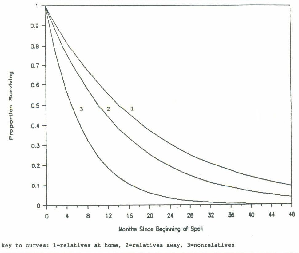
Figure 2 provides an additional illustration of the results. Here we see plotted survivor curves for three of the four types of child-care arrangements coded in the model: care by relatives at home, care by relatives away from home, and care by nonrelatives (the fourth type, center care, is not shown because its survivor curve is nearly coincident with that for relatives away from home). The probabilities used to compute these survival curves are those shown in Table 4. The curves indicate that the median length of nonrelative care (i.e. family day care), care by relatives away from home, and care provided by relatives in the child's home are about 6, 11, and 15 months, respectively.
| FIGURE 2. Survival Curves, Selected Types of Child Care |
 |
Basic Model of Entry
Results of logit estimates. Estimates of three alternative entry-into-child-care equations are shown in Table 5. Although the episodes analyzed here are defined by the use or nonuse of child care, it must be remembered that in most cases use of child care coincides with employment. Thus to some extent our child care entry equation is an employment entry equation.
Somewhat loosely, the explanatory variables investigated in this analysis fall into three categories; (1) subjective indices of the mother's perceptions of and information about barriers to obtaining child care, and of the mother's preferences for alternative child care arrangements; (2) the mother's potential market wage, theoretically of great importance in determining the woman's choice to work, and an unobserved attribute which must be imputed using auxiliary multivariate analyses; and (3) other fixed background and socioeconomic traits, many of which are in turn used to impute the potential market wage. The need to estimate an auxiliary wage function leads to an identification problem in the child-care entry equation, since at least one of the variables used in the wage-predicting equation must be excluded from the child care equation. There is an inherent arbitrariness in any exclusion used to identify the child care equation, and our experience suggests that the results obtained are rather sensitive to the choice of identifying restrictions. The results chosen for inclusion in Table 5 are fairly representative and "reasonable." However it should be acknowledged that equation (3) is the only one, among several alternatives that were tested, in which the predicted wage variable is statistically significant.
Equation (1) in Table 5 does not include the predicted wage variable, and does not include any variables used in computing the predicted wage. Most of the variables in equation (1) pertain to the preferences and perceptions indices of key interest in our analysis. The coefficients on ROD and CHOICE_5, both of which are positive and significant, appear to be counterintuitive. The first of these coefficients indicates that mothers who think that the type of care they most prefer is hard to obtain are, nonetheless, more likely than other mothers to begin a child care arrangement. The second can be interpreted similarly, since it shows that mothers whose preferred arrangement is center care, presumably a more demanding preference to satisfy than its less formal alternatives, have significantly higher probabilities of beginning a care arrangement.
| TABLE 5. Alternative Estimates of Entry-Into-Child Care Equation | |||
| Variable | Coefficient (Std. Err.) (1) | Coefficient (Std. Err.) (2) | Coefficient (Std. Err.) (3) |
| Constant | -6.773 (1.17) | -13.314 (4.11) | -7.515 (1.72) |
| HOWHARD | 0.122 (0.04)*** | 0.224 (0.06)*** | 0.172 (0.05)*** |
| CHOICE_5 | 1.397 (0.49)*** | 2.079 (0.83)** | 1.241 (0.59)** |
| KNOW_NO | -0.050 (0.36) | -1.890 (0.78)** | -1.149 (0.55)** |
| KNOW_DK | -2.873 (0.82)*** | -6.515 (1.71)*** | -3.175 (0.96)*** |
| RELSABLE | 1.074 (0.66) | -0.810 (1.04) | 0.606 (0.79) |
| AGEIND | -0.442 (0.15)*** | -1.334 (0.43)*** | -0.440 (0.19)** |
| JOBMOM | -1.189 (0.67)* | -2.157 (0.72)*** | |
| AFDCFAM | -1.676 (0.87)* | -0.814 (0.66) | |
| TEENMOM | -1.603 (0.84)* | -1.015 (0.77) | |
| BOSTON | -1.037 (1.11) | -1.253 (0.95) | |
| DENVER | 2.016 (0.96)** | -0.900 (0.88) | |
| TEENSIT | -0.787 (0.34)** | -0.188 (0.28) | |
| ADULTSIT | 0.041 (0.27) | 0.144 (0.22) | |
| BLACK | 9.527 (3.79)** | ||
| PWAGE | 0.373 (0.21)* | ||
| * significant at .10; ** significant at .05; *** significant at .01 | |||
A possible rationalization of the results for HOWHARD and for CHOICE_5 is that women with preferences and perceptions of this sort are better informed about the nature of the child care market, perhaps because they are actively engaged in search for a job and/or a child care arrangement. They may also have more previous experience of this market (a possibility which our data regrettably prevent us from testing). This "knowledge" interpretation happens to dovetail nicely with the results for the two indicators of lack of knowledge concerning the child- care reimbursement provisions of AFDC. Both of the AFDC knowledge indicators show that less-informed mothers are less likely to commence a child care episode, although the result is statistically significant [in equation (1)] only for the second of these two variables.
The coefficient on the child's age is negative, indicating a lower probability of beginning child care; this is the mirror image of the corresponding result in the exit equation, where it was found that the care arrangements of older children are relatively more likely to end.
Equation (2) adds a number of background characteristics to the equation, several of which turn out to be statistically significant. Three family-background factors--having grown up with a mother who worked, having grown up in a welfare family, and being a teenage mother oneself--all appear to inhibit entry into child care arrangements. But by far the largest effect in equation (2) is the race effect, which shows that black mothers are much more likely than mothers of other races to begin a child care arrangement.
Equation (3) is similar to equation (2), but it includes the predicted wage while excluding the race indicator. Based upon several unreported equations, it appears that only by excluding the race variable does the predicted wage become statistically significant. In general, however, the predicted wage has the theoretically anticipated sign (positive).
Implications of entry models. We have not included a table of illustrative probabilities, analogous to Table 4, in the case of the entry equations. The reason for this is the apparently highly skewed nature of the implied entry probabilities. When we substitute sample mean values (from Table 2) into an entry equation [in particular equation (2) in Table 5] we find that the "representative" per-period probability of beginning a child care episode is only 0.0001. Since the actual number of child care entries in the sample is 20, in a sample containing approximately 1200 "units" of exposure (i.e. 120 observations with an average of 10.4 periods per respondent in the sample) , the empirical average entry probability, while quite low, is nonetheless higher than 0.0001. A likely explanation for this situation is that the great majority of the sample has extremely low entry probabilities, while a small group has rather high probabilities; the logit model, a nonlinear model, appears not to capture the average of these two groups very well. Note that the average probability in the sample need not equal the probability attached to an average individual in this nonlinear model. Another possibility is that the estimates shown in Table 5 imply unexpectedly low average probabilities due to the failure of the estimates to control for unmeasured heterogeneity in the sample. Consequently we now turn briefly to a discussion of this issue.
Models With Unmeasured Heterogeneity
Our efforts to estimate the random-effects panel logit model described earlier, and represented by equations (3) through (5b), have so far met with only limited success. We have estimated variations on an exit model, one containing only two fixed covariates: JOBMOM and CONVENIENT. These are two variables which generally emerge as statistically significant in the simpler models presented earlier. The questions addressed in this exercise are (1) is there evidence of unmeasured heterogeneity, and does its presence in the model alter our conclusions about other measured variables? and (2) how does the model perform as we alter N, the (preset) parameter representing the number of points in the unmeasured-heterogeneity distribution?
Concerning the second of these questions, our limited experience to date suggests that the model is little affected by changes in N. The model (with two measured covariates as noted in the preceding paragraph) was estimated for N=1, N=2, and N=5. For these three variants, at least, the maximized value of the likelihood function changed only in the thousandths.
Parameter estimates for the second of these models (with N=2) are shown in Table 6.
The most immediately apparent findings in Table 6 are the enormous standard errors of the two parameters that represent unmeasured heterogeneity, r and §. Note that neither is estimated directly; rather, we estimate a logistic transform of r--that is, exp(r) / [1 + exp(r)]--in order to guarantee that r lies between 0 and 1, as required, and the natural logarithm of §, in order to impose the constraint §>0.
| TABLE 6. Results for Exit Model with Unmeasured Heterogeneity | |||
| Estimate | Standard Error | T-statistic | |
| logit (r) | 0.3329 | 208.794 | 0.002 |
| Constant (ß0) | -1.4483 | 0.585 | -2.477 |
| JOBMOM (ß1) | -0.1791 | 0.376 | -0.477 |
| CONVENIENT (ß2) | -0.3765 | 0.135 | -2.792 |
| ln (§) | -6.2209 | 148.718 | -0.042 |
In this model N=2, so that the possible values of z are 0 (with estimated probability f0 = .174), 1 (with probability f1 = .486) and 2 (with probability f2 = .339). These estimates suggest considerable diversity of the sample with respect to whatever unmeasured dimension is captured in the "z" term (if we disregard the extreme imprecision of the estimate of r). Yet these unmeasured differences do not seem to "matter", in the sense that the implied estimate of § is only 0.002, hardly enough to change exit probabilities noticeably. Together the findings from this limited exercise suggest, however tentatively, that unmeasured heterogeneity is not important in the analysis. Needless to say, this is an issue worthy of further investigation.
DISCUSSION
In this study we have investigated f actors associated with turnover in the child care arrangements of AFDC mothers. The phenomenon under study is an extremely complicated one, in view of the fact that welfare mothers seek child care arrangements in combination with a variety of productive activities including work, schooling or training programs, and job search. The correlates of entry into and exit from any of these types of activities therefore become, indirectly, correlates of turnover in child care arrangements. A further complication arises because each of these activities is linked to the process of entry to and exit from AFDC itself, which in turn alters the availability and net price of child care, and does so differently according to the type of care.
Our approach to these issues has been to simplify the problem in several respects, particularly by focusing simply upon the determinants of ending or beginning a child care arrangement, regardless of reason or type of concurrent activity.
A particular concern in our study has been to take account of mothers' preferences, perceptions, and knowledge about child care arrangements, both the actual arrangements used--among those in our sample observed to be using child care when interviewed--and potential arrangements--among those not using child care when interviewed, some of whom later began to use it.
The findings indicate that the mothers' perceptions are strongly related to their patterns of child care use. Among those using care when interviewed, those most satisfied with their care--measured with a four-point global satisfaction scale--had significantly lower probabilities of ending their child care arrangement per half-month period. A more disaggregated representation of satisfaction with care revealed that the convenience of the arrangement was the most important of several dimensions of satisfaction. Controlling for these scales, we found additional differentials in exit probabilities according to type of care: care by nonrelatives, which is in effect "family day care", emerged as significantly less durable arrangement than other types.
Considering those mothers not using child care when first interviewed, once again we found several indices of preferences and perceptions which appear to be significant predictors of entry into child care. An unexpected finding is that mothers who scored high on an index measuring their perceptions of the difficulty of finding satisfactory care were also more likely to begin a child care arrangement. Similarly, mothers whose most preferred type of care was center care-care in the formal service sector--were more likely to begin using care than were mothers preferring other types of arrangements.
Both these findings, however, seem consistent with an interpretation such, that better-informed mothers are more likely to use care. This interpretation is further supported by additional findings which show that women unaware of the child-care subsidy provisions of AFDC are less likely to begin using care than women who know about those provisions.
Our data do not, unfortunately, provide us with sufficient observations to make a systematic investigation into the agreement between stated preferences and the actual arrangements obtained. This would be an obvious area in which further investigations would be useful. Nonetheless, as they stand our findings seem to offer several insights into current child care policy issues. One is that policies which lower the cost of care will probably lead to more stable child care arrangements. Our "exit" equations consistently show that the higher the out-of-pocket cost of care, the greater is the likelihood that the care will end in a given period. However, the durability of child care would undoubtedly be enhanced either through lowering its cost, or through successful efforts to increase wage rates.
Another conclusion supported by our fin dings is that type of care may be less crucial than other attributes as an influence on the durability of care. Moreover, not all attributes appear to be equally important. For example, policies that succeed in raising adult/child ratios, or in mandating more stringent training or credentialing requirements on the part of providers, might contribute little to turnover patterns, at least within the welfare population, if they fail to lead to improved convenience as perceived by the mothers using the care. And, finally, it seems reasonable to conclude that the work behavior of welfare mothers would be promoted by policies which enhance those women's level of knowledge concerning the range of available child care services, and, equally important, the range of programmatic options open to them through the welfare program.
APPENDIX A: PREDICTED WAGE ANALYSIS
Our estimation of a predicted-wage equation uses data from the entire sample of women defined as "at risk" according to the criteria spelled out in the text. A wage equation was estimated using a subsample of at-risk women who were observed to have a wage rate at any point during the 14-month follow-up period of the study. Wherever possible we selected the wage rate observed at the start of an episode of employment. When this was not possible we controlled for the woman's tenure on the job for which the wage was observed. Using this approach we are able to predict a woman's starting wage were she to begin employment. The wage equation was estimated (in logarithmic form) using the "Mill's-ratio" approach to correction for subsample selectivity as outlined in Heckman (1976).
The estimates of both the selection and the wage equation are presented in Table A1. This table also includes the sample mean values for the variables used, for both the full sample (used-in the selection equation) and the subsample for which wages were observed.
The variables used in these equations include some not previously defined, including:
AGE -- respondent's age, in years.
AGESQ/100 -- respondent's age, squared (in 100s).
GRANDPAR -- a dummy variable indicating the presence in the household of the index child's grandparents).
YRS_ADDR -- the number of years the respondent has lived at her current address (as of the second interview).
YRS_AFDC -- the number of years the respondent has received AFDC in her lifetime (as of the second interview).
ED<12 -- a dummy variable indicating those with less than a high-school education.
ED=12 -- a dummy variable indicating those with exactly a high-school education.
ED>12 -- a dummy variable indicating those with more than 12 years of schooling (the omitted category pertains to those with missing information on years of education).
TENURE -- job tenure (in years) on the job currently held.
HOURS -- hours of work on the job currently held.
The variable LAMBDA appearing in the wage equation represents the Mill's ratio term used to correct the equation for sample selectivity. Although the wage equation estimated controls for both job tenure and hours of work, the predicted wage entered in the logistic regressions reported in the paper set tenure to zero and hours to 16; the former is done in order to represent entry-level wages, while the latter is done in order to standardize the wage for hours of work. Any fixed number of work hours could be used for this purpose, and the number 16 was chosen because it is close to the sample mean for those respondents actually observed to work.
| TABLE A1. Sample Means and Coefficient Estimates: Selection and Wage Equations | ||||
| Variable | Selection Equation | Ln (wage) Equation | ||
| Sample Mean | Coefficient (Std. Err.) | Sample Mean | Coefficient (Std. Err.) | |
| Constant | --- | 0.559 (0.70) | --- | 0.687 (0.37) |
| AFDCFAM | 0.53 | 0.300 (0.16)* | 0.54 | -0.182 (0.09)** |
| AGE | 27.34 | 0.004 (0.04) | 25.67 | 0.013 (0.02) |
| AGESQ/100 | 8.20 | -0.079 (0.07) | 7.13 | -0.005 (0.05) |
| JOBMOM | 0.31 | 0.150 (0.17) | 0.46 | 0.068 (0.09) |
| TEENSIT | 0.80 | -0.193 (0.08)** | --- | --- |
| ADULTSIT | 0.76 | 0.012 (0.09) | --- | --- |
| GRANDPAR | 0.22 | -0.203 (0.26) | --- | --- |
| YRS_ADDR | 4.08 | -0.006 (0.02) | 4.08 | -0.006 (0.01) |
| YRS_AFDC | 5.65 | 0.036 (0.02) | 5.48 | -0.024 (0.01)* |
| BOSTON | 0.25 | -0.010 (0.23) | 0.28 | 0.377 (0.12)*** |
| DENVER | 0.36 | -0.320 (0.22) | 0.30 | 0.491 (0.13)*** |
| AGEIND | 2.28 | 0.045 (0.05) | --- | --- |
| # CHILDREN | 1.88 | -0.194 (0.08)** | 1.75 | 0.058 (0.05) |
| ED<12 | 0.47 | -0.323 (0.32) | 0.44 | 0.041 (0.19) |
| ED=12 | 0.35 | -0.430 (0.33) | 0.33 | 0.320 (0.20) |
| ED>12 | 0.11 | 0.173 (0.38) | 0.15 | 0.144 (0.19) |
| TEENMOM | 0.71 | 0.140 (0.18) | 0.73 | 0.270 (0.10)*** |
| BLACK | 0.65 | 0.190 (0.18) | 0.70 | 0.297 (0.10)*** |
| HOURS | --- | --- | 16.40 | -0.001 (0.01) |
| TENURE | --- | --- | 0.11 | -0.042 (0.06) |
| LAMBDA | --- | --- | 0.821 | -0.425 (0.30) |
| Dependent Variable | 0.43 | --- | 1.29 | --- |
| * significant at .10; ** significant at .05; *** significant at .01 | ||||
REFERENCES
Allison, Paul 1982. "Discrete-Time Methods for the Analysis of Event Histories." In S. Leinhardt (ed.), Sociological Methodology 1982. San Francisco: Jossey-Bass.
Blau, David and Philip Robins (1988a) "Child Care Costs and Family Labor Supply." Review of Economics and Statistics LXX:374-381.
Blau, David and Philip Robins (1988b) "The Dynamics of Child Care Demand." Paper presented at the Winter Meetings of the Econometric Society, New York, December 1988.
Connelly, Rachel (1988) "Utilizing Market Child Care: An Economic Framework for Considering the Policy Issues." Unpublished manuscript.
Connelly, Rachel (1989) "The Effect of Child Care Costs on Married Women's Labor Force Participation." Unpublished manuscript.
Engberg, John, Peter Gottschalk and Douglas Wolf (1990) "A Random-Effects Logit Model of Work-Welfare Transitions." Journal of Econometrics 43: 63-75.
Floge, Liliane (1985) "The Dynamics of Child-care Use and Some Implications for Women's Employment." Journal of Marriage and the Family 47:143-54.
Heckman, James J. (1974) "Effects of Child-Care Programs on Women's Work Effort." Journal of Political Economy 82:S136-163.
Heckman, James J. (1976) "The Common Structure of Statistical Models of Truncation, Sample Selection, and Limited Dependent Variable Models and a Simple Estimator for Such Models" Journal of Economic and Social Measurement 5: 475-492.
Hofferth, Sandra L. and Douglas A. Wissoker (1990) "Quality, Price, and Income in Child Care Choice." Unpublished manuscript, The Urban Institute, February 1990.
Joesch, Jutta (1989) Labor Supply and the AFDC Child Care Subsidy: An Economic Analysis. Unpublished PhD Dissertation, Cornell University, August 1989.
Lehrer, E.L. (1983) "Determinants of Child Care Modal Choice: An Economic Perspective." Social Science Research 2: 69-80.
Robins, Philip K. and Robert Speigelman (1978) "An Econometric Model of the Demand for Child Care." Economic Inquiry XVI:83-94.
Sonenstein, Freya (1989) "The Child Care Preferences of Parents with Young Children: How Little is Known."
Sonenstein, Freya and Douglas A. Wolf (1988) "Caring for the Children of Welfare Mothers." Paper presented at the Annual Meetings of the Population Association of America, New Orleans, April 21-23 1988.
Sonenstein, Freya and Douglas A. Wolf (1990) "Characteristics of the Child Care Used by Welfare Mothers." Urban Institute report to DHHS/ASPE, May 1990.
Sonenstein, Freya and Douglas A. Wolf (forthcoming) "Parents' Child Care Preferences: Patterns Among Welfare Mothers" Journal of Social Issues. [Available at http://aspe.hhs.gov/daltcp/reports/ccpref.htm]
Wolf, Douglas A. (1987) "A Random-Effects Logit Model for Panel Data." Working Paper WP87-104. Luxemburg, Austria: International Institute for Applied Systems Analysis.
Yaeger, Kathryn (1979) "Cost, Convenience and Quality in Child Care Demand." Children and Youth Services Review 1: 293-313.