
Prepared by:
Julia Lane, Kelly S. Mikelson,
Patrick T. Sharkey, Douglas Wissoker
The Urban Institute
2100 M Street, NW
Washington, DC 20037
Submitted To:
U.S. Department of Health and Human Services
Office of the Assistant Secretary for Planning and Evaluation
Chapter 1: Introduction
The growth of alternative work arrangements temporary work, independent contractors, on-call workers, and contract company workers(5) has caught the attention of both policy makers and academic researchers alike. Part of the attention is due to the number of workers in the sector Bureau of Labor Statistics (BLS) data for the last five years indicate that 1 in 10 workers are employed in one of these four alternative work arrangements.(6) Another reason is the growth of the temporary help services industry. Employment in the temporary help services industry grew five times as fast as overall non-farm employment between 1972 and 1997 an average annual growth rate of 11 percent.(7) By the 1990s, this sector accounted for 20 percent of all employment growth.(8)
The growth of alternative work arrangements is important for another reason. The recent transformation of the nation's welfare system(9) combined with a strong economy has resulted in more individuals, many of whom have little employment experience, entering the labor force. However, our literature review shows that little is known about the importance of alternative work arrangements for these types of workers or the resulting labor market outcomes. This report attempts to fill the gap. The core research question was split into two components:
- How do alternative work arrangements differ from other arrangements in the characteristics of workers holding the jobs and in the characteristics of the jobs? How have these characteristics changed over time? What is the impact on low-income workers at risk of welfare recipiency? The part of the report that addresses this research question is primarily descriptive in nature, and structured to provide an environmental scan of the characteristics of the workers, jobs, and labor market outcomes.
- How do alternative work arrangements affect subsequent labor market outcomes for different types of workers particularly at-risk workers? The part of the report that addresses this research question is founded on a model-based approach that permits the construction of comparison groups and an analysis of possible counterfactual outcomes.
Two different sources of data are used: the Current Population Survey (CPS) for question 1, and the Survey of Income and Program Participation (SIPP) for question 2. Each is uniquely useful for each question. The CPS has rich detail to characterize the trends in and characteristics of alternative work arrangements in the mid- to late-1990s. The SIPP data from the 1990 through 1993 panels provide detailed work histories and the capacity to look at the impact of employment in temporary work on subsequent labor market outcomes one year later, including: employment status, hourly wages, weekly hours, private and employer-provided health insurance, public assistance receipt, Medicaid receipt, and poverty status.
The report is structured as follows. Chapter 2 provides an overview of the existing literature and research and sets the context for this study. In addition, Chapter 2 presents a first look at the evidence that is available from the existing literature both in terms of coming to grips with some of the definitional ambiguities and in terms of preliminary evidence on outcomes for workers in alternative work arrangements. Chapter 3 presents fresh evidence which describes the nature of alternative work arrangements, particularly with respect to the at-risk population, and is particularly focused on addressing the first part of the research question. Chapter 4 addresses the second part of the research question, examining the impact of alternative work arrangements specifically employment in the temporary help industry on workers in general and at-risk individuals in particular. Chapter 5 discusses the conclusions and implications drawn from the two different components of the study and discusses steps for future research.
5. These four alternative work arrangements independent contractors, on-call workers, temporary help agency workers, and workers provided by contract firms are taken from BLS' definition of alternative work arrangements.
6. Bureau of Labor Statistics. "Contingent and Alternative Employment Arrangements, February 1999." U.S. DOL/BLS. <ftp://ftp.bls.gov/pub/news.release/History/conemp.12211999.news>. December 1999; Bureau of Labor Statistics. "Contingent and Alternative Employment Arrangements, February 1997." U.S. DOL/BLS. <ftp://ftp.bls.gov/pub/news.release/History/conemp.020398.news>. December 1997; Bureau of Labor Statistics. "New Data on Contingent and Alternative Employment Examined by BLS." U.S. DOL/BLS. <ftp://ftp.bls.gov/pub/news.release/History/conemp.082595.news>. August 1995.
7. Autor, David H. "Outsourcing at Will: Unjust Dismissal Doctrine and the Growth of Temporary Help Employment," February, 2000; Estevao, Marcello M. and Saul Lach. "The Evolution of the Demand for Temporary Help Supply." NBER Working Paper No. 7427, December 1999.
8. Segal, Lewis M. and Daniel G. Sullivan. "The Growth of Temporary Services Work." Journal of Economic Perspectives Spring 1997b.
9. The Temporary Assistance for Needy Families (TANF) block grant, which was authorized in 1996 under the Personal Responsibility and Work Opportunity Reconciliation Act, emphasizes temporary assistance and a relatively fast transition to employment.
Chapter 2: A First Look at the Evidence
How did alternative work arrangements develop?
Although the terms contingent work and alternative work arrangements are relatively recent,(10) similar arrangements have existed for many decades or longer. The concept of temporary help services and workers dates to the late 1920s, and major temporary service firms began to operate shortly after World War II. Two of the largest temporary help services firms that still exist today--Manpower, Inc. and Kelly Girl, Inc.--were started in the late 1940s.(11) Manpower, Inc (established in 1948) is the largest temporary help services firm and is also the largest private employer in the country. With $11.5 billion in sales, Manpower employed 2.1 million employees worldwide in 1999.(12)
The literature suggests that firms have responded to market stimuli on both the demand and supply side. On the demand side, firms developed alternative work arrangements because technological advances and the consequent job specialization made it possible for firms to hire employees for specialized tasks rather than relying on employees with broad, generalized job descriptions. This had the additional advantage of allowing firms both to respond to the needs of consumers by expanding or contracting the size of the workforce and to change the mix of skills of employees. On the supply side, the increased number of women and young people in the workforce has increased the total number of workers in the labor force.(13) More total workers in the labor force results in more workers being available for flexible employment.
The literature also suggests that the development of alternative work arrangements has led to increased government regulation through labor law.(14) The past three decades have seen substantial changes to the common law doctrine "employment at will" which held that employers and employees have unlimited discretion to terminate the employment relationship at any time for any reason unless a contract exists stating otherwise. By 1995, 46 state courts limited employers' discretion to terminate workers, thus opening employers up to potentially costly litigation. The effect of state courts' changes to the employment-at-will doctrine explains up to 20 percent of the growth in the temporary help services industry, accounting for 336,000 to 494,000 additional workers daily in 1999.(15) It is possible that the legislative environment will change as a result of an August 2000 legislative decision by the National Labor Relations Board (NLRB) that expands collective bargaining rights for temporary help services employees. Although the impact of NLRB's ruling will not be known for some time, labor unions are already beginning to move to include agency temporaries in their membership.(16)
What are the different types of alternative work arrangements?
Alternative work arrangements are defined by the nature of the hiring arrangement between the worker and the employer.(17) The work provided by temporary help agencies is one example of these arrangements, while others include independent contractors, on-call workers and contract company workers. These are quite different types of work: for example, independent contractors might be real estate agents or freelance writers, while on-call workers include nurses, substitute teachers, and construction workers, and contract company workers include building security and cleaning workers and some computer programmers.(18)
It is worth examining the definition of temporary service work in more detail, both because it is quite complex and because it will be the focus of this report. The complexity is apparent in the conflicting estimates that come from worker-based surveys (the Current Population Survey (CPS)) and establishment-based surveys (the Current Employment Statistics survey (CES) and the Occupational Employment Statistics (OES) survey). In the CPS temporary help agency workers are those workers who said their job was temporary and answered affirmatively to the question, "Are you paid by a temporary help agency?" Workers who said their job was not temporary and answered affirmatively to the question, "Even though you told me your job was not temporary, are you paid by a temporary help agency?" are also included in the estimate of temporary help agency workers.(19) According to 1999 CPS data, approximately 1.2 million workers--about one percent of all workers--were temporary help agency workers. This estimate includes both workers placed by the temporary agency and a small amount of permanent full-time staff of these agencies--estimated to be about 3.2 percent of all workers employed by a temporary agency.(20)
In establishment-based surveys, such as the CES, the measure refers to the temporary help agency workers using the Standard Industrial Classification (SIC) code 7363--help supply services. Thus, while the CPS surveys people the CES surveys firms and, thus, counts the total number of temporary help services jobs. The help supply services code includes: "Establishments primarily engaged in supplying temporary or continuing help on a contract or fee basis. The help supplied is always on the payroll of the supplying establishments, but is under the direct or general supervision of the business to whom the help is furnished."(21) Thus, help supply services include employee leasing services workers and permanent staff at temporary help agencies as well as temporary help service workers. Because workers in employee leasing firms are not likely to resemble other agency temporaries, the presence of these firms within this classification makes comparisons using these data less reliable.(22)
Finally, it is worth noting that not all alternative work arrangements are transitory in nature. In fact, the Bureau of Labor Statistics makes a clear distinction between contingent work and alternative work arrangements, defining the former as: "Contingent work is any job in which an individual does not have an explicit or implicit contract for long-term employment or one in which the minimum hours worked can vary in a nonsystematic manner."(23) The difference is evident in an examination of Table 2.1 which indicates that although the majority of contingent workers are in alternative work arrangements, a small percentage of contingent workers are in traditional work arrangements, ranging from 3.2 to 3.6 percent from 1995 to 1999. Within the alternative work arrangement category there is substantial variation: independent contractors resemble workers in traditional arrangements and temporary help agency workers are at the other end of the spectrum.
| Arrangement | 1995 | 1997 | 1999 | |||||||||
|---|---|---|---|---|---|---|---|---|---|---|---|---|
| Contingent | Noncontingent | Contingent | Noncontingent | Contingent | Noncontingent | |||||||
| With alternative arrangements: | Number | % | Number | % | Number | % | Number | % | Number | % | Number | % |
| 316 | 3.8% | 7,993 | 96.2% | 296 | 3.5% | 8,160 | 96.5% | 239 | 2.9% | 8,008 | 97.1% |
| 792 | 38.1% | 1,286 | 61.9% | 533 | 26.7% | 1,463 | 73.3% | 569 | 28.0% | 1,463 | 72.0% |
| 785 | 66.5% | 396 | 33.5% | 738 | 56.8% | 562 | 43.2% | 664 | 55.9% | 524 | 44.1% |
| 129 | 19.8% | 523 | 80.2% | 135 | 16.7% | 674 | 83.3% | 155 | 20.2% | 614 | 79.8% |
| With traditional arrangements(c) | 3,998 | 3.6% | 107,054 | 96.4% | 3,883 | 3.4% | 110,316 | 96.6% | 3,811 | 3.2% | 115,298 | 96.8% |
| Total | 6,020 | 4.9% | 117,252 | 95.1% | 5,585 | 4.4% | 121,175 | 95.6% | 5,439 | 4.1% | 125,906 | 95.9% |
| Source: Bureau of Labor Statistics. a. For this table we use the broadest definition of contingent work which includes workers who do not expect their jobs to last. The self-employed and independent contractors are included if they expect their emploiyment to last for an additional year or less and they had been self-employed or independent contractors for 1 year or less. b. Noncontingent workers are those who do not fall into any estimate of contingent workers. c. Workers with traditional arrangements are those who do not fall into any of the alternative arrangements categories. | ||||||||||||
Why do firms use alternative work arrangements?
The reasons for firms to use alternative work arrangements are almost as varied as the different types of these arrangements. Firms elect to use workers in alternative work arrangements for a variety of reasons. Cost effectiveness is one: contingent employment and alternative work arrangements enable employers to lower wages and benefit costs. Another is the flexibility provided by contingent workers that allows employers to expand and contract their workforce with the economy. Researchers have also suggested that employers use temporary help agencies to screen workers for permanent positions, thereby reducing turnover costs and training costs.(24)
Several surveys of employers have been conducted in recent years to better understand employer use of alternative work arrangements--the most recent is a nationally representative survey of employers conducted by the Upjohn Institute for Employment Research.(25) This survey of 550 private sector employers with five or more employees asked firms questions about their use of the following alternative work arrangements: agency temporaries, on-call workers, independent contractors, short-term hires,(26) and regular part-time workers. We will limit our discussion to those work arrangements previously defined as alternative: agency temporaries, on-call workers, and independent contractors. Upjohn gathered information on (1) which employers use flexible staffing arrangements; (2) how much these employers use them; (3) why they use them; (4) how the wages and benefits of flexible workers compare to traditional workers; and (5) whether employers have increased or decreased their relative use of these arrangements since 1990, and if so, why.(27)
The first finding is that the use of alternative workers is pervasive, but varies by firm size and industry. As shown in Table 2.2, Houseman (1997) reports that the Upjohn Survey found that 27 percent of surveyed firms used on-call workers, 46 percent used agency temporaries, and 44 percent used contract workers in 1995. Between 1990 and 1995, the overall percentage of firms using on-call workers and agency temporaries stayed about the same, with equal shares of firms increasing and decreasing their use of such arrangements. Houseman also reports that the incidence of alternative work arrangements increases with firm size. However, even among small firms (with five to nine employees), use of such arrangements is non-negligible. Approximately one-sixth of small firms used agency temporaries and on-call workers, while one-third used contract workers. The industry variation is substantial: 72 percent of manufacturing firms used agency temporaries, while the use of on-call workers was highest in the services industry (44 percent), and the incidence of contract workers was highest in the mining and construction industries (see Table 2.2) (Houseman, 1997).
| On-call Workers | Temporary Help Agency Workers | Contract Workers | |
|---|---|---|---|
| Firms using alternative workers | |||
| Use | 27.3% | 46.0% | 43.5% |
| Dont use | 72.4% | 53.5% | 54.7% |
| Dont know | 0.4% | 0.5% | 1.8% |
| Firms reported change in use of alternative workers since 1990 | |||
| Increased | 17.3% | 24.3% | NA |
| Decreased | 15.3% | 23.9% | NA |
| Remained about the same | 64.7% | 47.8% | NA |
| Dont know | 2.7% | 4.0% | NA |
| Industries using alternative workers | |||
| Agriculture | 13.0% | 50.0% | 25.0% |
| Mining/Construction | 11.0% | 56.0% | 61.0% |
| Manufacturing | 13.0% | 72.0% | 54.0% |
| Transportation, Public Utilities, and Communications | 21.0% | 50.0% | 54.0% |
| Trade | 16.0% | 37.0% | 34.0% |
| Services | 44.0% | 44.0% | 47.0% |
| Source: Houseman 1997. | |||
Houseman (1997) provides empirical evidence as to why firms use alternative work arrangements. The Upjohn Institute survey(28) showed that the reasons vary by work arrangement, but staffing reasons are more frequently cited than others (see Table 2.3). Firms most often use on-call workers and agency temporaries to fill in for an absent employee who is sick, on vacation, or on family medical leave or to provide needed assistance at times of unexpected increases in business. Firms also report frequently using agency temporaries to fill a vacancy until a regular employee is hired, while a smaller percentage of firms hire temporary or on-call workers to meet seasonal fluctuations in their workload.
| On-call Workers | Temporary Help Agency Workers | |
|---|---|---|
| Staffing reasons for using alternative workers | ||
| Fill vacancy until regular employee is hired | 26.0% | 46.6% |
| Fill in for absent regular employee who is sick, on vacation, or on family medical leave | 69.3% | 47.0% |
| Seasonal needs | 29.3% | 28.1% |
| Provide needed assistance during peak-time hours of the day or week | 37.3% | 14.2% |
| Provide needed assistance at times of unexpected increases in business | 50.7% | 52.2% |
| Special projects | 26.0% | 36.0% |
| Other reasons for using alternative workers | ||
| Screen job candidates for regular jobs | 8.0% | 21.3% |
| Save on wage and/or benefit costs | 6.0% | 11.5% |
| Provide needed assistance during company restructuring or merger | 6.0% | 7.5% |
| Fill positions with temporary agency workers for more than one year | NA | 5.1% |
| Save on training costs | NA | 5.1% |
| Special expertise possessed by this type of worker | 16.0% | 10.3% |
| Source: Houseman 1997. | ||
The screening hypothesis is not borne out by the empirical evidence--firms are less likely to cite non-staffing reasons for hiring on-call workers and agency temporaries. Only one in five firms hires agency temporaries to screen them for regular jobs, and only 8 percent of firms hire on-call workers to screen them for permanent positions. On-call workers were used by about 16 percent of firms for their special expertise, while agency temporaries were used by about 10 percent of firms for their expertise.
Although saving on wage and/or benefit costs has often been cited as an important reason for the use of workers in alternative work arrangements, the evidence in Table 2.3 does not support this. In fact, as Table 2.4 shows, most firms report that hourly pay costs are about the same for on-call workers as regular workers in similar positions while hourly pay costs are actually higher for agency temporaries for the majority of firms. The story changes somewhat when benefit costs are added to the hourly pay costs. Nearly three-quarters of firms say their costs for on-call workers are lower than benefit and wage costs for regular workers in a similar position. On the other hand, firms report that their costs for agency temporaries are about the same or lower than benefit and wage costs for regular workers in similar positions. However, firms may still be saving money overall since the flexibility of alternative work arrangements allows them to hire workers for short-term needs.
| On-call Workers | Temporary Help Agency Workers | |
|---|---|---|
| Firms hourly pay cost for alternative workers(a) | ||
| Higher than regular workers | 16.7% | 62.1% |
| Lower than regular workers | 18.7% | 13.4% |
| About the same as regular workers | 61.3% | 21.7% |
| Don't know | 3.3% | 2.8% |
Firms hourly pay plus benefit cost for alternative workers(b) | ||
| Higher than regular workers | 5.3% | 19.4% |
| Lower than regular workers | 72.7% | 38.3% |
| About the same as regular workers | 19.3% | 38.3% |
| Don't know | 2.7% | 4.0% |
| Source: Houseman 1997. a. For temporary help agency workers, the comparison was between the hourly billed rate for temporary help agency workers and the hourly pay cost of regular employees in comparable positions. b. For temporary help agency workers, the comparison was between the hourly billed rate for temporary help agency workers and the hourly pay plus benefit cost of regular employees in comparable positions. | ||
In sum, the empirical evidence suggests that while there are many reasons for firms to use alternative work arrangements, firms' staffing needs--primarily short term--are the main source of demand for on-call workers and agency temporaries. Firms do not often use alternative work arrangements to screen employees for full-time, permanent positions--although some firms do use these workers for their special expertise in a particular area. And, only five percent of companies report hiring agency temporaries to save on training costs. The cost savings in terms of wages and benefits are also not a major element in firms' decisions, as shown by the small percentages of firms that cite such savings as a reason for hiring temporaries or on-call workers.
How many workers are in alternative work arrangements, and who are they?
The Contingent Work supplement to the CPS in 1995, 1997, and 1999 splits employment into eight mutually exclusive groups--Independent contractors, on-call workers, temporary help agency workers, contract company workers, direct-hire temporary workers, regular self-employed (excluding independent contractors), regular part-time workers, and regular full-time workers. The first four categories of these are alternative work arrangements. As is clear from Table 2.5, the proportion of workers in temporary help services is approximately one percent, and has not changed substantially in the past five years. Although the proportion of workers in alternative work arrangements is higher if the definition is broadened--particularly if on-call workers are included--there is no discernable trend from these data. This stands in marked contrast to estimates derived from using establishment-based data (Table 2.6), which suggest that temporary help employment grew from 1.4 percent of total employment in 1991 to almost 3 percent of total employment by 1999. The reasons for this discrepancy are not fully understood by the Bureau of Labor Statistics, which publishes both series, so here we are unable to do more than simply note the difference.(29)
| 1995 | 1997 | 1999 | ||||
|---|---|---|---|---|---|---|
| Type of Employment Arrangement | Number | Percent | Number | Percent | Number | Percent |
| Independent contractors Workers who were identified as independent contractors, independent consultants, or freelance workers, whether they were self-employed or wage and salary workers. | 8,309 | 6.7 | 8,456 | 6.7 | 8,247 | 6.3 |
| On-call workers Workers who are hired directly by an organization, but work only on an as-needed basis when they are called to do so, for example, substitute teachers, construction workers, and some types of hospital workers. | 2,078 | 1.7 | 2,023 | 1.6 | 2,032 | 1.7 |
| Temporary help agency workers Workers who said their job was temporary and answered affirmatively to the question, Are you pad by a temporary help agency? Also, workers who said their job was not temporary and answered affirmatively to the question, Even though you told me your job was temporary, are you pad by a temporary help agency? Thus, these estimates may include the small number of permanent staff of these agencies. | 1,181 | 1.0 | 1,300 | 1.0 | 1,188 | 0.9 |
| Contract company workers Workers who are employed by a company that contracted out their services, if they were usually assigned to only one customer, and if they generally worked at the customerme types of hospital workers. | 588 | 0.5 | 763 | 0.6 | 769 | 0.5 |
| Direct-hire temporaries Workers in a job temporarily for an economic reason and who are hired directly by a company rather than through a staffing intermediary. | 3,393 | 2.8 | 3,263 | 2.6 | 3,227 | 2.5 |
| Regular self-employed Workers who identified themselves as self-employed (incorporated and unincorporated) who were not independent contractors. | 7,256 | 5.9 | 6,510 | 5.1 | 6,280 | 4.8 |
Regular part-time | 16,810 | 13.7 | 17,290 | 13.6 | 17,380 | 13.2 |
| Regular full-time Individuals not in one of the other categories above who usually work 35 hours or more per week. | 83,600 | 67.9 | 87,140 | 68.8 | 92,222 | 70.1 |
| Total | 123,215 | 100 | 126,745 | 100 | 131,345 | 100 |
| Source: Bureau of Labor Statistics. | ||||||
| Year | Employment in Temporary Help Services (in thousands) | Total Private NonFarm Employment (in thousands) | Temporary Help as Percent of All Employment |
|---|---|---|---|
| 1991 | 1,268 | 89,847 | 1.41% |
| 1992 | 1,411 | 89,956 | 1.57 |
| 1993 | 1,669 | 91,872 | 1.82 |
| 1994 | 2,017 | 95,036 | 2.12 |
| 1995 | 2,189 | 97,885 | 2.24 |
| 1996 | 2,352 | 100,189 | 2.35 |
| 1997 | 2,656 | 103,133 | 2.58 |
| 1998 | 2,926 | 106,042 | 2.76 |
| 1999 | 3,228 | 108,616 | 2.97 |
Source: Current Employment Statistics, Bureau of Labor Statistics | |||
Not surprisingly, there is as much heterogeneity in the workers in alternative work arrangements as in the types of these arrangements and the reasons for firms using them. As Table 2.7 shows, according to 1999 BLS data, independent contractors are the most prevalent of the alternative work arrangements at 6.3 percent of all workers. Independent contractors are more likely to be white (91 percent) and male (66 percent) than traditional workers, who are 84 percent white and 52 percent male. On average, independent contractors are more often part-timers and are marginally more educated than workers in traditional work arrangements. Over half of independent contractors are in two industries--construction (20 percent) and services (42 percent).
| Characteristic | Workers with Traditional Arrangements(a) | Independent Contractors | On-Call Workers | Temporary Help Agency Workers | Contract Workers | |
|---|---|---|---|---|---|---|
| Total, 16 years and over | 119,109 | 8,247 | 2,032 | 1,188 | 769 | |
| Percent | 90.6% | 6.3% | 1.5% | 0.9% | 0.6% | |
| Gender | ||||||
| Men, 16 years and over | 52.4% | 66.2% | 48.8% | 42.2% | 70.5% | |
| Women, 16 years and over | 47.6% | 33.8% | 51.2% | 57.8% | 29.5% | |
| Race and Hispanic Origin(b) | ||||||
| White | 84.0% | 90.6% | 84.2% | 74.3% | 79.2% | |
| Black | 11.4% | 5.8% | 12.7% | 21.2% | 12.6% | |
| Hispanic | 10.4% | 6.1% | 11.6% | 13.6% | 6.0% | |
| Full- and Part-time Status | ||||||
| Full-time workers | 82.9% | 75.1% | 49.3% | 78.5% | 86.8% | |
| Part-time workers | 17.1% | 27.9% | 50.7% | 21.5% | 13.2% | |
| Educational Attainment | ||||||
| Less than a high school diploma | 9.2% | 7.5% | 13.4% | 14.6% | 6.4% | |
| High school graduates, no college | 31.4% | 29.7% | 29.6% | 30.5% | 22.7% | |
| Less than a bachelor's degree | 28.3% | 28.5% | 29.1% | 33.7% | 31.9% | |
| College graduates | 31.1% | 34.3% | 27.9% | 21.2% | 38.9% | |
| Median Earnings | ||||||
| Median usual weekly earnings,16 years and over | $540 | $640 | $472 | $342 | $756 | |
| Preference for Traditional Work Arrangement | ||||||
| Prefer traditional arrangement | NA | 8.5% | 46.7% | 57.0% | NA | |
| Prefer indirect or alternative arrangement | NA | 83.8% | 44.7% | 33.1% | NA | |
| It depends | NA | 5.2% | 4.8% | 5.3% | NA | |
| Not available | NA | 2.5% | 3.8% | 4.6% | NA | |
| Industry | ||||||
| Agriculture | 2.0% | 4.9% | 2.2% | 0.4% | 0.4% | |
| Mining | 0.4% | 0.2% | 0.4% | 0.1% | 2.7% | |
| Construction | 5.1% | 19.9% | 9.6% | 2.5% | 9.0% | |
| Manufacturing | 16.5% | 4.6% | 4.5% | 29.7% | 18.0% | |
| Transportation and public utilities | 7.4% | 5.7% | 9.5% | 6.1% | 14.0% | |
| Wholesale trade | 4.0% | 3.5% | 1.8% | 4.2% | 0.8% | |
| Retail trade | 17.6% | 10.2% | 14.6% | 3.9% | 4.6% | |
| Finance, insurance, and real estate | 6.7% | 8.8% | 2.7% | 7.0% | 8.9% | |
| Services | 35.2% | 42.1% | 52.0% | 38.7% | 27.1% | |
| Public Administration | 5.1% | 0.2% | 2.6% | (c) | 10.7% | |
| Not reported or ascertained | 0.0% | 0.0% | 0.1% | 6.3% | 3.8% | |
| Occupation | ||||||
| Executive, administrative, and managerial | 14.6% | 20.5% | 5.3% | 4.3% | 12.0% | |
| Professional specialty | 15.5% | 18.5% | 24.3% | 6.8% | 28.8% | |
| Technicians and related support | 3.3% | 1.1% | 4.1% | 4.1% | 6.7% | |
| Sales occupations | 12.0% | 17.3% | 5.7% | 1.8% | 1.5% | |
| Administrative support, including clerical | 15.0% | 3.4% | 8.2% | 36.1% | 3.4% | |
| Services | 13.7% | 8.8% | 23.5% | 8.1% | 18.8% | |
| Precision production, craft, and repair | 10.5% | 18.9% | 10.1% | 8.7% | 16.0% | |
| Operators, fabricators, and laborers | 13.6% | 7.0% | 16.0% | 29.2% | 10.7% | |
| Farming, forestry, and fishing | 2.0% | 4.4% | 2.9% | 0.9% | 2.2% | |
| Source: BLS 1999. a. Workers with traditional arrangements are those who do not fall into any of the racteristics, February 1999. b. Detail for the above race and Hispanic-origin groups will not sum to totals because data for the ruary 1999. c. Less than 0.05 percent. NA = Not Available. | ||||||
On-call workers are second most common and have a gender and racial distribution similar to that of traditional workers. However, half of on-call workers work part time compared to 17 percent of workers in traditional arrangements. On average, on-call workers are somewhat less educated than traditional workers with 13 percent having less than a high school diploma compared to 9 percent of traditional workers. Half of on-call workers work in the service industry with the most likely occupations being professional specialty (e.g., teachers, lawyers, engineers, architects) (24 percent) and services (24 percent).
Agency temporaries, who comprise nearly one percent of all workers, are more likely than the average worker to be female (58 percent compared to 48 percent of traditional workers), black (21 percent compared to 11 percent), and Hispanic (14 percent compared to 10 percent). Agency temporaries are the least educated group of workers, on average, and 79 percent are full-time workers, compared to 83 percent of traditional workers. Not surprisingly, nearly 40 percent of agency temporaries work in the services industry, compared to 35 percent of traditional workers, with the most common occupations among agency temporaries being administrative support and clerical positions (36 percent).
The smallest group of alternative workers is contract workers--0.6 percent of all workers. Contract workers, like independent contractors, are more likely to be men (71 percent) than traditional workers (52 percent) but have a similar racial distribution to traditional workers. Contract workers are somewhat more likely than any other group to be full-time workers (87 percent) compared to traditional workers (83 percent), the next highest group. On average, contract workers are more educated than those in any other work arrangement--39 percent of contract workers are college graduates, compared to 31 percent of workers in traditional arrangements.
A First Look at How Labor Market Outcomes Differ For Workers In Alternative Work Arrangements
No single definitive statement can summarize the impact of alternative work on employees. The impact depends on the factors mentioned above: the kind of work arrangement the worker is in, the reason the firm hired the worker, and the demographic characteristics of the worker. The type of work arrangement may also affect many elements of a worker's labor market experience including earnings, job tenure, health insurance coverage, and pension benefits. And, although it is natural to compare the outcomes of alternative work arrangements with those resulting from regular work, this may not be appropriate for some demographic groups such as those for whom the alternative may be nonemployment or welfare receipt. An argument can be made that people who would otherwise be on public assistance or receiving unemployment insurance are better off working in an alternative work arrangement.
Earnings
Earnings in this sector tend to be lower than for traditional work (although this depends on the type of arrangement). As Table 2.7 indicates, in 1999, the median of earnings for workers in traditional arrangements was $540 per week. This was significantly higher than the median earnings of agency temporaries at $342 per week--nearly $200 per week lower than traditional workers--and on-call workers at $472 per week. Contract workers earned more than workers in any other arrangement with $756 in median weekly earnings in 1999. Independent contractors earned $100 more than workers in traditional arrangements, with $640 in median weekly earnings.
It is possible that differences in educational attainment or in the total hours worked per week contribute to these aggregate discrepancies in earnings. On-call workers and agency temporaries have the lowest educational attainment while independent contractor and contract workers are most highly educated, indicating a strong correlation between earnings and education. In addition, contract workers are more likely than any other group to be working full-time. Full- or part-time status cannot explain all the gaps in earnings, however, since agency temporaries are the second most likely to be working full-time and they have the lowest median weekly earnings.
In a study that controlled for some of these differences, Segal and Sullivan (1998)(30) find that a 15 to 20 percent wage differential exists between wages earned in temporary work and the wages that would be expected from traditional work based on the work history of the individuals in the sample. This differential dropped to about 10 percent when wages were compared to those earned at the types of jobs that the individuals would probably find if not involved in temporary work.
Benefits
In general, one disadvantage to alternative work arrangements is the lack of health insurance and employer-provided pension plans. Indeed, Farber (1997) uses the presence or absence of such plans as one of his measures of "good" or "bad" jobs.(31) While workers in all alternative work arrangements are less likely to have health insurance and pension plans than workers in traditional arrangements, the coverage varies quite a bit by alternative arrangement. As Table 2.8 indicates, BLS data show that 83 percent of workers in traditional arrangements have health insurance coverage and 58 percent have coverage provided by their employer. While contract workers have nearly the same health insurance and pension plans as workers in traditional arrangements, other alternative work arrangements provide health insurance coverage and pension plans less frequently. In terms of health insurance, agency temporaries are the worst off, since only 41 percent have health insurance from any source and 9 percent have employer-provided insurance. Two-thirds of on-call workers have health care coverage from any source and one-fifth receive health care coverage from their employer. Nearly three-quarters of independent contractors have health insurance; however, it is never supplied by the employer.
| Characteristic | Percent with health insurance coverage | Percent eligible for employer-provided pension plan | ||
|---|---|---|---|---|
| Total | Provided by employer | Total | Included in employer-provided pension plan | |
With traditional arrangements | 82.8% | 57.9% | 54.1% | 48.3% |
| With alternative arrangements | ||||
| Independent contractors | 73.3% | NA | 2.8% | 1.9% |
| On-call workers | 67.3% | 21.1% | 29.0% | 22.5% |
| Temporary help agency workers | 41.0% | 8.5% | 11.8% | 5.8% |
| Contract workers | 79.9% | 56.1% | 53.9% | 40.2% |
| Source: BLS 1999. NA = Not applicable. | ||||
Fifty-four percent of workers in traditional arrangements are eligible for an employer-provided pension plan and nearly half are included in their employer's pension plan (see Table 2.8). Again, contract workers most closely resemble workers in traditional work arrangements with 54 percent eligible for an employer-provided pension plan and 40 percent included in that plan. Only 12 percent of agency temporaries are eligible for an employer-provided pension plan and 6 percent are actually included. Independent contractors fare the worst in employer-provided pensions with 3 percent eligible and 2 percent actually included. Thus, health insurance coverage and employer-provided pensions are provided less frequently to workers in alternative work arrangements, and many workers must purchase these amenities on their own if they wish to be covered.
Job Tenure
Evidence indicates that, with the exception of independent contractors, job tenure in alternative work arrangements is shorter than in traditional arrangements. The median tenure (in the arrangement) for independent contractors was 7.7 years, according to 1997 CPS data, while traditional arrangements had a median tenure of 4.8 years. Temporary help agency workers had the shortest tenure with six months, and on-call workers and contract workers both had a median tenure of 2.1 years in 1997.(32) This is reinforced by Segal and Sullivan's (1997a) research, which finds that temporary employment spells are dramatically shorter than permanent spells. Their estimates lead them to conclude that 32 percent of temporary employment spells for one employer last for only one quarter (compared to 11 percent of permanent spells), 78 percent last four quarters or fewer (compared to 35 percent of permanent spells), and the average is about two quarters.
Job Satisfaction
As Table 2.9 shows, in 1997, independent contractors, on-call workers, and agency temporaries reported vastly different reasons for their decision to work in alternative arrangements. Independent contractors were much more likely to cite personal reasons(33) (76 percent) over economic reasons(34) (9 percent). Among independent contractors working in an alternative arrangement for a personal reason, flexibility of schedule was the most commonly cited reason. On-call workers were split nearly evenly between personal reasons (41 percent) and economic reasons (39 percent). Of on-call workers citing economic reasons, most said it was the only type of work they could find while those citing personal reasons most often cited flexibility of schedule as the primary reason. Agency temporaries, on the other hand, were more than twice as likely to cite economic reasons (60 percent) as they were to cite personal reasons (29 percent). Temporary workers most often said that this was the only type of work they could find and that they hoped this job leads to a permanent position.(35)
| Reason | Independent Contractors | On-Call Workers | Temporary Help Agency Workers |
|---|---|---|---|
| Total, 16 years and over (in thousands) | 8,456 | 1,996 | 1,300 |
| Percent | 100.0% | 100.0% | 100.0% |
Economic reason | 9.4% | 40.7% | 59.6% |
| Only type of work I could find | 2.7% | 27.1% | 34.6% |
| Hope job leads to permanent employment | 0.7% | 5.3% | 17.7% |
| Other economic reason | 6.0% | 8.3% | 7.2% |
Personal reason | 76.0% | 39.4% | 29.3% |
| Flexibility of schedule | 23.6% | 22.4% | 16.1% |
| Family or personal obligations | 3.9% | 6.0% | 2.4% |
| In school or training | 0.6% | 6.4% | 4.5% |
| Other personal reason | 48.0% | 4.6% | 6.4% |
Reason not available | 14.6% | 19.9% | 11.1% |
| Source: Cohany 1998. Note: Information for contract workers was not available. | |||
Summing Up
Given the evidence about earnings, job tenure, health insurance coverage, pension benefits, preference for traditional employment, and reasons for working in alternative arrangements, it is clear that the advantages and disadvantages to alternative work vary by work arrangement. Earnings, health coverage, and employer-provided pensions are common among independent contractors and contract workers while many on-call workers and agency temporaries lack these benefits and, on average, have low median earnings. Independent contractors also report preference for their alternative arrangement while on-call workers are split and agency temporaries report strong preference for a traditional arrangement. Finally, agency temporaries cite economic reasons for alternative employment while on-call workers are split and independent contractors cite personal reasons. We can conclude from this that independent contractors and contract workers are much more likely to enter alternative work arrangements willingly and to benefit financially from work more than agency temporaries and somewhat more than on-call workers. The heterogeneity among positions using an alternative work arrangement is reflected in the heterogeneity of the effects on the well-being of the workers.
A First Look at How Alternative Work Arrangements Affect Low-Income and At-Risk Workers
In order to address this core research question, it is necessary to define low-income and at-risk workers. Unfortunately, there is no clear consensus on either definition. In defining low income or low wage, income from many different sources (e.g., wages, public assistance, child support), over many different time periods (e.g., hourly, weekly, annually), and many different units (e.g., individual, family, household) may be considered (see Theeuwes, Lane, and Stevens 2000; Brown 1999; Dickert-Conlin and Holtz-Eakin 1999; Hudson 1999). Different thresholds are often used as well: some absolute, such as a multiple of the minimum wage (see Brown 1999) or wages necessary to lift a family of four above the poverty threshold (see Hudson 1999)., and some relative, such as the relative position in the income distribution (e.g., lowest 20 percent of the income distribution) (See Theeuwes, Lane, and Stevens 2000; Dickert-Conlin and Holtz-Eakin 1999; and Hudson 1999). There is similarly no clear definition of at risk of welfare recipiency because of the wide variety of income eligibility rules for TANF in each state. Thirty-six of 50 states have a gross income test--income before deductions and disregards, resulting in an income variation ranging from $616 (Oregon) to $1,955 (Alaska) in monthly income,(36) (37) or if translated into poverty thresholds, a range of from 56 to 177 percent of the 1999 poverty threshold for a family of three. Similar variation occurs if we consider Medicaid income eligibility which translates into a range between 48 and 209 percent of the 1999 federal poverty threshold, although the national threshold for food stamps is 135 percent of poverty level. In any event, the gross monthly income limits for the three major public assistance programs range from 48 to 209 percent of the 1999 federal poverty threshold.
Can the terms low wage, low income, and at risk of welfare recipiency be used synonymously? Research by Dickert-Conlin and Holtz-Eakin (1999) suggests that low-wage workers and poor workers are not the same, and, in fact, only 15 percent of low-wage workers--with wages below $5.93--the lowest quintile of the wage distribution--are poor. They also find that poor workers are much more likely than low-wage workers to receive public assistance. Twenty percent of poor workers receive public assistance while only about 7 percent of low-wage workers receive some form of public assistance. This is not surprising given the lower incomes of households with poor workers ($9,431) compared to households with low-wage workers ($38,384). Thus, a definition of low income that is based on the poverty level is much more likely--although by no means certain--to include individuals at risk of welfare recipiency than a definition of low income that is based on wage rates.
No CPS-based study has focused exclusively on low-income workers in alternative work arrangements, possibly because of the small number of workers in alternative arrangements. As Table 2.10 shows, the number of public assistance recipients in alternative work arrangements nationwide is rather small. However, there is some evidence that workers in alternative work arrangements are over-represented among low-wage workers and workers with incomes below or near the poverty line.(38) In a recent study analyzing the 1999 February CPS,(39) GAO found that about 8 percent of standard full-time workers had annual family incomes below $15,000, as compared with 30 percent among agency temporaries. Likewise, GAO found that nearly every category of alternative workers--including agency temporaries, direct-hire temporaries, on-call workers, independent contractors, and part-time workers--had a greater percentage of workers with family incomes below $15,000. In fact, only self-employed and contract workers had a lower or similar percentage of workers with family incomes below $15,000 annually.(40)
Work Arrangement | Total Number (weighted) | Percent of All Workers (weighted) |
|---|---|---|
| Agency Temporaries | 198,460 | 2.2% |
| On-call Workers | 290,840 | 3.6% |
| Contract Company Workers | 60,054 | 0.7% |
| Self-employed | 731,460 | 8.2% |
| Regular Workers | 7,681,000 | 85.7% |
| Source: Current Population Survey February Supplement, 1999. Note: Percentages may total to more than 100 due to rounding. | ||
Houseman (1999) used the February Supplement to the 1997 CPS and matched files for the February and March 1995 CPS to analyze both hourly wages and poverty levels for workers in alternative arrangements compared to regular employees. This descriptive data analysis(41) uses the 1997 CPS data to calculate the percentage of workers earning at or near the minimum wage--between $4.25 and $5.15 in 1997. She finds that some workers in alternative arrangements do better than regular employees while others do worse.(42)
There is evidence from Unemployment Insurance (UI) wage record data that temporary help jobs for welfare recipients are not of high quality. Pawasarat (1997) examines over 42,000 jobs held between January 1996 through March 1997 by over 18,000 single parents who received Aid to Families with Dependent Children (AFDC) benefits in December 1995. In particular, Pawasarat found that temporary help jobs were often part time or short term: of those hired by a temporary agency over the five quarters, only 30 percent used that agency as the sole source of employment. Additionally, earnings were low. Between 48 and 52 percent of those employed by temporary employment agencies earned under $500 per quarter in wages. Only 9 to 13 percent of the temporary workers earned the equivalent of a full-time salary (at least $2500) in a temporary job in a given quarter.
However, he finds that temporary agencies provide an entry point into the labor market for AFDC recipients, and are important in a numerical sense. In particular, he finds that 30 percent of all jobs held by these workers were concentrated in temporary agencies compared to 23 percent in retail trade, and that over the five quarters studied, 42 percent of AFDC recipients who had a job were employed at least once by a temporary agency.
It is certainly clear that a greater percentage of agency temporaries, on-call workers, and other short-term direct hires earn near the minimum wage than do regular employees (Table 2.11). These low wages translate into low family incomes and thus a greater percentage of workers in alternative arrangements earn below or near the poverty line as compared with regular workers. Furthermore, since workers in alternative work arrangements are more likely to work intermittently or for fewer than full-time hours, it is not surprising that their overall incomes are lower than those of regular employees.
| Hourly Wage $4.25-$5.15(a) | Percent Below Poverty(b) | Percent Near Poverty (100%-125% of Poverty Line)(b) | |
|---|---|---|---|
| Working Arrangement | |||
| Agency Temporaries | 9.3% | 14.2% | 7.5% |
| On-call or Day Laborers | 13.9% | 12.0% | 4.2% |
| Independent Contractors | 4.3% | 7.7% | 3.1% |
| Contract Company Workers | 5.5% | 6.7% | 4.8% |
| Other Short-term Direct Hires | 17.9% | 10.9% | 4.2% |
| Other Self-employed | 6.0% | 7.5% | 2.3% |
| Regular Employees | 7.0% | 4.8% | 2.7% |
| Source: Houseman 1999. a. Tabulations from the February 1997 CPS Supplement on Contingent and Alternative Work Arrangements. b. Tabulations from matched data from the February 1995 and March 1995 CPS. | |||
These findings are reinforced by Houseman's (1997) analysis of the February 1995 CPS. She finds that workers in alternative work arrangements are much more likely to receive low wages, live in poverty, and have no benefits, than are workers in regular full-time jobs. Further evidence indicates that while workers in alternative work arrangements account for about 25 percent of wage and salary workers, they account for 57 percent of those in the bottom ten percent of the wage distribution, 56 percent of those not eligible to receive employer-provided health insurance, and 42 percent of the working poor.(43)
Despite the evidence that workers in alternative work arrangements are more likely to have earnings below the poverty line, it would be premature to conclude that low-income alternative workers are hurt by their alternative work arrangements. It is not clear that without these alternative work arrangements these workers would be better off since many might be unemployed or discouraged workers, particularly in view of the low levels of human capital held by these workers.
A First Look at Whether Alternative Work Arrangements Help Workers On The Path To Regular Employment
Some TANF agencies have begun using temporary help agencies to help place welfare recipients in jobs.(44) This may well become an important trend--as more former welfare recipients go to work and the caseload becomes harder to serve, welfare agencies are likely to rely more heavily on intermediaries that either provide services to help clients with employment barriers (e.g., substance abuse treatment) or assist with job search activities including teaching clients "soft skills" necessary to succeed in interviews. While this may be helpful to some workers with few skills and little or no work history, opponents fear that the temporary agency jobs are low paying with only a small chance of the job becoming a permanent position.(45)
Survey-based evidence suggests that few temporary jobs lead to permanent employment--only 5 percent of companies report hiring agency temporaries to fill positions for more than one year. A recent study using CPS data confirms that there is a significant amount of job turnover for agency temporaries. In an analysis of labor market transitions for personnel supply services workers (SIC 736) between 1983 and 1993, Segal (1996) found that half of personnel supply services workers were employed in a different industry after one year. In each year between 1983 and 1993, on average, 20 percent of those who were personnel supply services workers in the preceding year were without a job in the subsequent year, either out of the labor force (13.8 percent) or unemployed (6.3 percent).(46)
UI wage record data also suggest that few temporary jobs become permanent. In Washington, fewer than half of temporary employment spells (42 percent) result in a transition to a permanent job (Segal and Sullivan 1997a). In Wisconsin, only 5 percent of the single parents who worked for temporary agencies at any point in the five quarters had nontemporary agency earnings over $2500 during the first quarter of 1997. Roughly 6 percent of persons with temporary agency jobs may have obtained full-time nontemporary employment through a temporary job. Most of these successful persons had the characteristics of the population most likely to leave AFDC with or without a temporary job placement, i.e., 69 percent had 12 or more years of schooling and 57 percent were already employed in first quarter 1996 at the start of the study period.(47) In addition, even after controlling for demographic characteristics as well as work and welfare histories, the Pawasarat (1997) study generally found significantly lower probabilities of working in all four quarters in the year after leaving welfare if a welfare recipient had worked in a temporary agency as compared to other industries.
Although most jobs do not convert to permanent jobs, some firms do provide the opportunity. The Upjohn Institute's survey found that about 43 percent of employers using agency temporaries and 36 percent of employers using on-call workers said they often, occasionally, or sometimes move employees into permanent positions. This is confirmed by a survey conducted by the National Association of Temporary Staffing Services, which found that more than one-third of temporary agency workers surveyed said they had been offered a permanent job by their employers.(48)
10. Polivka, Anne E. "Contingent and Alternative Work Arrangements, Defined." Monthly Labor Review, October 1996b.
11. Moore, Mack A. "The Temporary Help Service Industry: Historical Development, Operation, and Scope." Industrial Labor Relations Review, 1965.
12. Manpower Inc. "Manpower Inc. Facts." Manpower Inc. <http://www.manpower.com/en/story.asp>. 2000.
13. Lee, Dwight R. "Why Is Flexible Employment Increasing?" Journal of Labor Research XVII, no. 4, Fall 1996: 543-53.
14. Autor 2000; Lee 1996.
15. Autor 2000.
16. Swoboda, Frank. "Temporary Workers Win Benefits Ruling." The Washington Post, August 31 2000, A1.
17. It is worth making the point that there is a difference between contingent work and alternative work arrangements: the latter describe the relationship between employer and employee, the former is closely tied to the expected duration of employment
18. Cohany, Sharon R. "Workers in Alternative Employment Arrangements." Monthly Labor Review October 1996.
19. Cohany 1996.
20. Houseman, Susan N. and Anne E. Polivka. "The Implications of Flexible Staffing Arrangements for Job Stability." Upjohn Institute Staff Working Paper No. 99-056, May 1999.
21. U.S. Department of Labor. "SIC Description for 7363." Occupational Safety and Health Administration. <http://www.osha.gov/cgi-bin/sic/sicser2?7363>. 2000.
22. Typically a company will contract with an employee leasing firm and then dismiss their employees only to have them hired by the leasing company and leased back to the original firm. The leasing company provides wages, payroll taxes, and benefits to the employees for a set fee. See KRA Corporation. Employee Leasing: Implications for State Unemployment Insurance Programs. Unemployment Insurance Service, Department of Labor, 1996.
23. Polivka, Anne E. and Thomas Nardone. "On the Definition of 'Contingent Work'." Monthly Labor Review December 1989.
24. Abraham, Katherine G. and Susan K. Taylor, "Firms' Use of Outside Contractors: Theory and Evidence" Journal of Labor Economics, July 1996: 394-424.
25. Houseman, Susan N. "Temporary, Part-Time, and Contract Employment in the United States: A Report on the W.E. Upjohn Institute's Employer Survey on Flexible Staffing Policies." U.S. Department of Labor. June 1997.
26. The Upjohn Survey defines short-term hires as individuals who are employed directly by the organization for a limited and specific period of time. Short-term hires include workers hired for the December holiday season or during the summer and they may work part-time hours.
27. Houseman 1997.
28. The Upjohn Institute survey reports establishment responses about alternative work arrangements. Thus, the perspectives of alternative workers are not reflected in these data. Also, the averages in the data represent the typical firm, rather than the firm whether the typical worker is located.
29. It is worth discussing the discrepancy between these results and those reported based on establishment employment statistics in some detail. The Current Population Survey (CPS), which covers households, and the Current Employment Statistics survey (CES), which covers firms, do not agree on the level of employment in the United States for a number of reasons, but primarily because the former series covers workers and the latter covers jobs. However, in the 1990s the gap between the two series grew markedly: employment as measured by the CPS grew by only 8 million (from 110 million to 118 million) from 1994 to 1998 while the CES showed an employment growth of more than 12 million (from 113 million to over 125 million) (Nardone 1999). The reason for this discrepancy is not known--it could be due to changes in multiple job holding, undocumented illegal immigration, Census undercounts (and hence misweighting in the CPS), or changes in establishment reporting practices. Although understanding the causes for these differences has important implications for knowing how much true employment growth has actually occurred in the temporary help sector, and is an important area for future research, it is beyond the scope of the current study.
30. The authors use Unemployment Insurance (UI) data from the State of Washington to examine wage differentials and employment duration, respectively, among workers in the temporary help supply services industry.
31. Farber, Henry S. "Job Creation in the United States: Good Jobs or Bad?" Princeton University Industrial Relations Section Working Paper 385, July 1997.
32. Cohany, Sharon R. "Workers in Alternative Employment Arrangements: A Second Look." Monthly Labor Review November 1998.
33. Personal reasons, as defined in the CPS, include: flexibility of schedule; family or personal obligations; in school or training; and other.
34. Economic reasons, as defined in the CPS, include: employer laid off and hired back as temporary employee, only type of work I could find, hope job leads to permanent employment, retired/social security earnings limit, nature of work/seasonal, and other.
35. Cohany 1998.
36. Center for Law and Social Policy and Center on Budget and Policy Priorities. "State Policy Demonstration Project." <www.spdp.org/medicaid/table_3.htm>. January 2000.
37. For reasons of comparison, we selected gross income limits and the 1999 poverty threshold for a family of three.
38. U.S. General Accounting Office. "Contingent Workers: Incomes and Benefits Lag Behind Those of Rest of Workforce." GAO/HEHS-00-76, June 2000; Houseman, Susan N. "Flexible Staffing Arrangements: A Report on Temporary Help, On-Call, Direct-Hire Temporary, Leased, Contract Company, and Independent Contractor Employment in the United States." DRAFT, June 1999; Houseman 1997.
39. All of the studies with income information for alternative workers discussed here rely on data from the February Contingent Workers and Alternative Work Arrangements supplement to the CPS or March CPS.
40. U.S. GAO 2000a.
41. This paper provides descriptive statistics; the estimates do not control for other factors that may affect human capital.
42. Houseman's definition of "regular employees" is not clear from the paper, however, it likely refers to workers in traditional arrangements and may or may not include part-time employees along with full-time employees.
43. Houseman 1997.
44. Pavetti, LaDonna, Michelle Derr, Jacquelyn Anderson, Carole Trippe, and Sidnee Paschal. The Role of Intermediaries in Linking TANF Recipients with Jobs. Mathematica Policy Research, Inc. U.S. DHHS/ASPE, February 2000; Houseman 1999.
45. Houseman 1999.
46. Segal, Lewis M. "Flexible Employment: Composition and Trends." Journal of Labor Research XVII, no. 4 Fall 1996: 523-42. See Table 6 on page 539.
47. Pawasarat, John. "The Employment Perspective: Jobs Held by the Milwaukee County AFDC Single Parent Population (January 1996-March 1997). Milwaukee, WI: Employment and Training Institute, December 1997.
48. Houseman 1997.
Chapter 3: New Evidence for At-Risk and Low-Income Workers in Alternative Work Arrangements
It is clear from Chapter 2 that both definitional issues and the key research questions are complex--so we should expect the examination of new evidence to be equally complex. This is indeed the case. We use two different sources of data to examine the research questions.(49) In this chapter we exploit the Current Population Survey to address the first component of the research question, namely: how do labor market outcomes for at-risk workers in alternative work arrangements compare with those of all workers and low-income workers in traditional employment. The reason for the use of the CPS is that it is an excellent source for describing a variety of different work arrangements as well as for using different measures of at risk. Consequently, the CPS provides quite rich detail to characterize the trends in and characteristics of alternative work arrangements.
One of the main issues faced with using the CPS was that very few individuals were both at risk and working in alternative work arrangements. Table 3.1 shows the sample sizes associated with the most feasible definitions of at-risk or low-income individuals--namely, individuals who had received public assistance in the previous period, who had a family income below 150 percent of the poverty line, or who had a family income below 200 percent of the poverty line. (50)
|
Work Arrangement |
1995 | 1997 | 1999 |
|---|---|---|---|
|
All Workers |
|||
| Agency Temps | 342 | 347 | 322 |
| On-Call Workers | 671 | 632 | 679 |
| Regular Workers | 34,934 | 31,970 | 32,470 |
|
Public Assistance Recipients |
|||
| Agency Temps | 77 | 52 | 73 |
| On-Call Workers | 90 | 93 | 118 |
| Regular Workers | 3,445 | 3,296 | 2,785 |
|
Workers Below 150% Poverty |
|||
| Agency Temps | 99 | 82 | 94 |
| On-Call Workers | 135 | 140 | 133 |
| Regular Workers | 3,874 | 3,565 | 3,254 |
|
Source: Current Population Survey, matched February to March. |
|||
Characteristics of At-Risk Workers In Alternative Work Arrangements
Our examination of the CPS data reveals that workers who are at risk of welfare recipiency by either of our two definitions are more than twice as likely to be in alternative work arrangements as are other workers (Table 3.2). Although there appears to be no observable trend in the proportions of either former public assistance recipients or workers from poor families who are agency temps, there is a slight increase in the proportion of the former who are on-call workers.(51)
Work Arrangement | 1995 | 1997 | 1999 |
|---|---|---|---|
All Workers | |||
| Agency Temps | 0.8% | 1.0% | 0.9% |
| On-Call Workers | 1.6 | 1.6 | 1.7 |
| Regular Workers | 84.1 | 84.9 | 85.9 |
Public Assistance Recipients | |||
| Agency Temps | 2.2% | 1.4% | 2.3% |
| On-Call Workers | 2.1 | 2.2 | 3.2 |
| Regular Workers | 85.6 | 86.8 | 85.6 |
Workers Below 150% Poverty | |||
| Agency Temps | 2.5% | 2.2% | 2.3% |
| On-Call Workers | 2.9 | 3.2 | 3.2 |
| Regular Workers | 79.9 | 82.2 | 80.7 |
Source: Current Population Survey, matched February to March | |||
It is worth noting that at-risk workers who get jobs in alternative work arrangements do not differ much from at-risk workers who get standard jobs--they have similar education levels and age distributions (Table 3.3). However, the education level of these workers is very low--over one-third are high school dropouts; three out of four have a high school education level or less. The only salient difference is the sex of the workers: in 1995, over half of at-risk temporary workers were male, but by 1999, this had fallen to less than one-third. In comparison, among at-risk workers in regular employment, roughly 44 percent were male, and this remained relatively unchanged between 1995 and 1999. There are some substantial differences in the industry in which at-risk workers work, however. In particular, at-risk workers in temporary help employment are almost twice as likely to be employed in the service sector than at-risk workers in regular employment, and one sixth as likely to be in trade.
| 1995 | 1997 | 1999 | |||||||
|---|---|---|---|---|---|---|---|---|---|
| agency temps | on-call workers | regular workers | agency temps | on-call workers | regular workers | agency temps | on-call workers | regular workers | |
| Age | |||||||||
| 16-24 | 24.3% | 20.4% | 25.8% | 29.4% | 26.1% | 25.7% | 33.4% | 27.6% | 25.7% |
| 25-54 | 64.9 | 69.0 | 66.8 | 65.1 | 61.0 | 67.2 | 62.6 | 61.8 | 67.2 |
Sex | |||||||||
| Male | 51.2% | 42.9% | 46.6% | 50.8% | 46.3% | 45.9% | 30.8% | 48.0% | 43.9% |
Education | |||||||||
| Less than HS Diploma | 33.5% | 26.4% | 30.8% | 25.5% | 33.2% | 28.8% | 29.5% | 36.5% | 29.4% |
| HS Diploma | 43.2 | 33.8 | 38.5 | 36.8 | 41.2 | 40.4 | 38.1 | 35.4 | 37.3 |
Number of Jobs Held | |||||||||
| More than one | 8.1% | 8.9% | 5.5% | 7.7% | 5.9% | 5.2% | 5.1% | 5.2% | 4.5% |
Industries | |||||||||
| ag/mining/fishing | 2.4% | 7.4% | 3.7% | 2.0% | 7.9% | 4.0% | 1.1% | 14.5% | 2.7% |
| construction | 5.6 | 16.1 | 5.4 | 1.8 | 20.3 | 4.7 | 4.5 | 10.0 | 5.3 |
| manufacturing | 24.5 | 6.8 | 15.6 | 21.0 | 9.4 | 16.0 | 26.4 | 3.4 | 14.2 |
| transp/commun/utils | 4.0 | 2.4 | 4.6 | 2.1 | 2.0 | 4.1 | 2.6 | 3.8 | 5.2 |
| trade | 5.8 | 17.4 | 30.6 | 6.2 | 15.6 | 31.6 | 1.2 | 19.5 | 32.4 |
| services | 57.0 | 44.9 | 35.5 | 65.4 | 38.2 | 36.4 | 63.2 | 41.0 | 37.0 |
| other | 0.7 | 5.0 | 4.5 | 1.6 | 6.6 | 3.2 | 0.9 | 7.8 | 3.2 |
Source: Current Population Survey, matched February to March | |||||||||
Where are the jobs?
If we list the major industries that hire temporary workers (not just at-risk temporary workers), it is clear that the business services and auto and repair services industries are overwhelmingly important demanders of temporary labor--accounting for roughly half of all temporary help employment (See Table 3.4). However, most of this is accounted for by personnel supply services (Table 3.5), which in turn lease out the workers to other industries. In addition, durable goods manufacturing accounts for just over one in ten jobs for temporary help workers, and employment in other professional services another one in twenty. In examining those industries (at a finer level of industrial detail) that employ temporary help workers (Table 3.6), other important users of temporary help worker services are health services, hospitals, telephone communications, electrical machinery, equipment and supplies and computer and data processing services. There are few discernable trends in these patterns over the five-year period for which we have data.
Industry | % of Agency Temps in 1995 | % of Agency Temps in 1997 | % of Agency Temps in 1999 |
|---|---|---|---|
| Agriculture | 0.5% | 1.0% | 0.3% |
| Mining | 0.5 | 0.9 | 0.0 |
| Construction | 3.1 | 1.0 | 2.4 |
| Manufacturing - Durable Goods | 11.9 | 10.9 | 14.7 |
| Mfg. - Non-Durable Goods | 7.5 | 7.2 | 6.6 |
| Transportation | 2.4 | 3.1 | 1.3 |
| Communications | 2.1 | 1.3 | 1.0 |
| Utilities And Sanitary Services | 0.3 | 0.6 | 0.5 |
| Wholesale Trade | 1.4 | 2.5 | 1.8 |
| Retail Trade | 1.9 | 1.1 | 1.6 |
| Finance, Insurance, And Real Estate | 1.8 | 4.7 | 2.8 |
| Private Households | 0.8 | 0.6 | 0.5 |
| Business, Auto And Repair Services | 55.2 | 50.1 | 53.0 |
| Personal Services, Exc. Private Hhlds | 0.7 | 0.4 | 1.2 |
| Entertainment And Recreation Services | 0.7 | 0.6 | 0.3 |
| Hospitals | 0.4 | 1.8 | 1.3 |
| Medical Services, Exc. Hospitals | 2.8 | 5.6 | 3.7 |
| Educational Services | 2.2 | 0.2 | 0.7 |
| Social Services | 1.0 | 1.1 | 0.3 |
| Other Professional Services | 2.4 | 5.3 | 4.6 |
| Forestry And Fisheries | 0.0 | 0.0 | 0.0 |
| Public Administration | 0.5 | 0.0 | 1.2 |
| Armed Forces | 0.0 | 0.0 | 0.0 |
Source: Current Population Survey matched February to March. | |||
| Year | Detailed Industry | Census Code | % of Business, Auto and Repair Services Temps |
|---|---|---|---|
| 1995 | Personnel Supply Services | 731 | 35.2% |
| Elec machinery, equip, and supplies, n.e.c. | 342 | 3.3 | |
| Computer and Data Processing Services | 732 | 3.0 | |
| Unknown | 999 | 3.0 | |
| Credit agencies, n.e.c. | 702 | 2.6 | |
| Construction | 60 | 2.4 | |
| Banking | 700 | 2.3 | |
| Insurance | 711 | 2.1 | |
| 1997 | Personnel Supply Services | 731 | 49.7% |
| Computer and Data Processing Services | 732 | 7.2 | |
| Business services, n.e.c. | 741 | 3.7 | |
| Soaps and cosmetics | 182 | 2.4 | |
| Motor vehicle and motor vehicle equipment | 351 | 2.3 | |
| Unknown | 999 | 2.2 | |
| Construction | 60 | 2.0 | |
| 1999 | Personnel Supply Services | 731 | 36.4% |
| Hospitals | 831 | 5.4 | |
| Computer and Data Processing Services | 732 | 4.7 | |
| Elec machinery, equip, and supplies, n.e.c. | 342 | 3.3 | |
| Telephone communications | 441 | 3.3 | |
| Insurance | 711 | 2.8 | |
| Business services, n.e.c. | 741 | 2.8 | |
| Unknown | 999 | 2.5 | |
| Detective and protective services | 740 | 2.4 | |
Source: Current Population Survey matched February to March. | |||
| Year | Detailed Industry | Census Code | % of Agency Temps | Median Education Level Among All Temps | Median Education Level Among All Workers |
|---|---|---|---|---|---|
| 1995 | Personnel supply services* | 731 | 19.4% | HS Grad | Some College |
| Electrical machinery, equipment, and supplies | 342 | 4.7 | HS Grad | Some College | |
| Construction | 60 | 4.4 | HS Grad | HS Grad | |
| Telephone communications | 441 | 2.6 | Some College | Some College | |
| 1997 | Personnel supply services | 731 | 24.9% | HS Grad | Some College |
| Health services | 840 | 4.8 | Some College | College Grad | |
| Computer and data processing services | 732 | 3.6 | College Grad | College Grad | |
| Motor vehicles and motor vehicle equipment | 351 | 2.8 | Some College | HS Grad | |
| Machinery, except electrical | 331 | 2.5 | HS Grad | HS Grad | |
| 1999 | Personnel supply services | 731 | 19.3% | HS Grad | Some College |
| Hospitals | 831 | 4.2 | College Grad | College Grad | |
| Health services | 840 | 3.7 | HS Grad | College Grad | |
| Electrical machinery, equipment, and supplies | 342 | 3.1 | Some College | Some College | |
| Telephone communications | 441 | 2.7 | Some College | Some College | |
| Computer and data processing services | 732 | 2.5 | Some College | College Grad | |
Source: Current Population Survey, matched February to March | |||||
A detailed industry analysis reveals that the number of industries drawing on temporary help workers has increased, and that the median education level of temporary workers employed in these industries is quite high. In almost all of the industries in 1997 and 1999 (but not 1995), the median education level of workers is beyond high school, and in some (notably telephone communications and computer and data processing services), the median worker is a college graduate. It is also worth noting that there appears to be some increased demand for higher education qualifications among temporary help workers. All the "newly important" industries that emerge by 1999--namely, telephone communications and hospitals--have more temporary help workers with at least some college than not; the one "important" industry in 1995 that was no longer important by 1999 was construction, which had more high school graduates and dropouts than not. This trend stands in marked contrast to the average education level of the at-risk group in which we are interested (Table 3.3), where only about one in four workers has education beyond a high school diploma, as described previously. Finally, while the median temporary worker is usually less educated than the median regular worker in the firm that hires her, the level of skill required for the temporary job is usually below that of the median regular worker. This introduces the possibility that as skill levels in the economy as a whole increase, so will the demand for the skills of temporary help workers, with clear implications for at-risk temporary workers, who are generally less educated.
Although only a few industries account for the bulk of temporary worker hiring, the dominance of just a few sectors is less evident when the occupational distribution of temporary help workers is examined. As Table 3.7 shows, a large number of workers classify themselves as working in administrative support occupations (almost one in three), but we also see large numbers working as machine operators, assemblers, inspectors, handlers, equipment cleaners, helpers, and laborers.
| Occupation | % of Agency Temps in 1995 | % of Agency Temps in 1997 | % of Agency Temps in 1999 |
|---|---|---|---|
| Executive, Admin, & Managerial Occs | 6.0% | 7.7% | 4.5% |
| Professional Specialty Occs | 8.6 | 7.4 | 6.8 |
| Technicians And Related Support Occs | 3.8 | 6.2 | 4.1 |
| Sales Occs | 3.1 | 1.4 | 1.6 |
| Admin. Support Occs, Incl. Clerical | 29.2 | 31.2 | 34.7 |
| Private Household Occs | 0.6 | 0.3 | 0.0 |
| Protective Service Occs | 1.6 | 0.9 | 1.3 |
| Service Occs, Exc. Protective & Hhld | 5.7 | 8.3 | 7.2 |
| Precision Prod., Craft & Repair Occs | 7.2 | 4.9 | 9.3 |
| Machine Opers, Assemblers & Inspectors | 17.9 | 19.3 | 19.5 |
| Transportation And Material Moving Occs | 3.0 | 2.8 | 2.0 |
| Handlers,equip Cleaners,helpers,labors | 12.6 | 7.7 | 8.5 |
| Farming, Forestry And Fishing Occs | 0.7 | 2.0 | 0.7 |
| Armed Forces | 0.0 | 0.0 | 0.0 |
| Source: Current Population Survey matched February to March. | |||
Again, turning to examine the occupations of temporary help workers in more detail, as Table 3.8 shows, it is clear that in 1995, the median education level of most temporary help workers in these occupations was quite low, and the occupations were fairly unskilled: laborers, secretaries, data entry keyers, assemblers, typists, nursing aides, and the like. However, just as the "newly important" industries in Table 3.6 employed a more highly educated temporary worker, on average, in 1999 than did the industries in 1995, so too did the educational mix of temporary workers in "important" occupations change by 1999. For example, bookkeepers, accounting and auditing clerks--an occupation in which the median temporary help worker had some college--appeared as an important occupation by 1999.
| Year | Detailed Occupation | Census Code | % of Agency Temps | Median Education Level Among All Temps | Median Education Level Among All Workers |
|---|---|---|---|---|---|
| 1995 | Laborers, except construction | 889 | 6.9% | HS Grad | HS Grad |
| Secretaries | 313 | 6.6 | Some College | HS Grad | |
| Assemblers | 785 | 6.2 | HS Grad | HS Grad | |
| Data entry keyers | 385 | 5.1 | HS Grad | Some College | |
| Typists | 315 | 2.8 | HS Grad | Some College | |
| Receptionists | 319 | 2.5 | HS Grad | HS Grad | |
| Industrial truck and tractor equipment operators | 856 | 2.5 | HS Grad | HS Grad | |
| 1997 | Secretaries | 313 | 8.2% | Some College | Some College |
| Assemblers | 785 | 5.5 | HS Grad | HS Grad | |
| Nursing aides, orderlies, and attendants | 447 | 5.0 | HS Grad | HS Grad | |
| Laborers, except construction | 889 | 4.7 | HS Grad | HS Grad | |
| General office clerks | 379 | 3.8 | Some College | Some College | |
| File clerks | 335 | 2.8 | Some College | HS Grad | |
| 1999 | Assemblers | 785 | 7.0% | Some College | HS Grad |
| Nursing aides, orderlies, and attendants | 447 | 5.1 | HS Grad | HS Grad | |
| Laborers, except construction | 889 | 5.0 | Some College | HS Grad | |
| Secretaries | 313 | 4.8 | Some College | Some College | |
| Bookkeepers, accounting, and auditing clerks | 337 | 3.9 | Some College | Some College | |
| Data entry keyers | 385 | 3.7 | Some College | HS Grad | |
| File clerks | 335 | 2.9 | HS Grad | HS Grad | |
| Machine operators, not specified | 779 | 2.7 | HS Grad | HS Grad | |
Source: Current Population Survey matched February to March. | |||||
In general, just as with the industry analysis, the type of temporary help worker that is needed appears to be changing. In 1995, the education level of temporary help workers matched the education level of the regular workers in their occupations. By 1999, the median temporary help worker's education exceeded that of regular workers in three of the eight most important occupations. Indeed, the median education level for temporary help workers in five of these eight occupations was "some college," which is well above the education level of at-risk temporary workers.
The Characteristics of Jobs for At-Risk Workers in Alternative Work Arrangements
Although temporary help jobs have often been characterized as peripheral and marginal in nature, little is known about whether these jobs are substantially different for at-risk workers than for the workforce in general. This section examines several different aspects of jobs in the alternative work arrangements sector--the quantity of work (hours and job duration), the price of work (the wage rate), and other measures of the quality of work (such as benefit information). Although these measures are of interest in any analysis of the labor market, they are of particular interest to those at risk of welfare receipt. It is self-evident that low wages are an important contributing factor to poverty--and it is also well known that the difference between low-wage workers below poverty and low-wage workers above poverty is the number of weeks and hours worked per year. (52) In addition, work by Farber (1997) shows that the availability of health and pension benefits for low-skill workers is steadily decreasing, lowering the quality of jobs available to this group.
Part-time Employment and Job Duration
A number of quite interesting facts emerge from an examination of the evidence on part-time employment and job duration presented in Table 3.9. The first set of rows, for all workers, reveal that the rate of part-time work is much higher for workers in alternative work arrangements than those in regular employment, and job tenure is shorter. Although fewer than one in six regular workers works part time, more than one in five agency temps, and roughly one in two on-call workers work under 30 hours a week. Similarly, although nine in ten regular workers have been in their jobs more than six months, only slightly more than half of agency temps have been, and three out of four on-call workers. This has already been well documented by Polivka (1996a), and is not surprising, given the inherently transient and part-time nature of both temporary and on-call employment. It is interesting to note, however, that there has been no discernable change in this pattern over the past five years.
| Work Arrangement | 1995 | 1997 | 1999 | ||||||
|---|---|---|---|---|---|---|---|---|---|
| Part-Time | Job Tenure | Part-Time | Job Tenure | Part-Time | Job Tenure | ||||
| % Part-Time | % More Than 6 Months | %More Than One Year | % Part-Time | % More Than 6 Months | % More Than One Year | % Part-Time | % More Than 6 Months | % More Than One Year | |
| All Workers | |||||||||
| Agency Temps | 21.4% | 54.5% | 38.8% | 19.2% | 57.6% | 39.1% | 20.6% | 59.9% | 43.6% |
| On-Call Workers | 55.7 | 73.6 | 61.5 | 49.6 | 75.1 | 63.5 | 51.7 | 72.1 | 62.1 |
| Regular Workers | 16.9 | 90.0 | 81.5 | 16.6 | 89.9 | 81.8 | 15.7 | 90.2 | 81.6 |
| Public Assistance Recipients | |||||||||
| Agency Temps | 22.8% | 48.4% | 37.4% | 25.2% | 54.0% | 35.2% | 29.3% | 52.2% | 32.4% |
| On-Call Workers | 60.3 | 71.1 | 46.6 | 49.5 | 65.2 | 48.0 | 55.2 | 69.6 | 66.0 |
| Regular Workers | 24.3 | 81.0 | 67.4 | 23.2 | 82.4 | 69.7 | 23.4 | 82.7 | 69.4 |
| Workers Below 150% Poverty | |||||||||
| Agency Temps | 26.2% | 52.2% | 39.1% | 20.2% | 44.7% | 31.3% | 26.0% | 50.7% | 29.0% |
| On-Call Workers | 56.5 | 63.5 | 49.0 | 58.0 | 62.9 | 47.5 | 52.4 | 58.1 | 50.5 |
| Regular Workers | 28.5 | 75.5 | 59.9 | 29.5 | 78.0 | 63.7 | 27.9 | 77.5 | 62.3 |
Source: Current Population Survey, matched February to March. | |||||||||
When we turn to examine whether similar part-time patterns hold true for at-risk workers in alternative work arrangements versus at-risk workers in regular employment (the second and third sets of rows in Table 3.9), it is clear that at-risk workers are more likely to be part time than are all workers across the board, regardless of what kind of job they hold. However, this increased likelihood of part-time work is greater for at-risk workers in regular jobs than for at-risk workers in either temporary work or on-call work.
In keeping with this finding, it is also clear from Table 3.9 that job duration in general is also lower for at-risk workers in alternative work arrangements regardless of whether the comparison group is their cohort in regular work or all other agency temps. If we compare at-risk workers who are agency temps with at-risk workers who have regular employment, only about one in two at-risk workers who are agency temps have been in their job more than six months, while eight in ten at-risk workers who have regular employment have been in their job at least six months. If we compare at-risk agency temps to other agency temps, it is clear that the proportion of at-risk workers with job tenure greater than either six months or one year is generally less than other agency temps. All of these groups have much lower job duration than do regular workers in general, where nine in ten have a job that has lasted at least six months, and eight in ten have a job that has lasted at least one year.
Finally, there appears to have been little change in these patterns over time--there is little evidence of a trend in the data. Neither the rate of part-time work nor job duration has changed substantially--and this holds true both for all workers and for those at risk of welfare receipt.
Wages
The second component of job quality in which we are interested is wages. It is clear from Table 3.10 that earnings of workers in alternative work arrangements are substantially below those in regular work, although average earnings in this sector have showed a slightly stronger upward trend than overall earnings.
| Work Arrangement | 1995 | 1997 | 1999 | |||
|---|---|---|---|---|---|---|
| Mean Wage | Median Wage | Mean Wage | Median Wage | Mean Wage | Median Wage | |
All Workers | ||||||
| Agency Temps | $9.32 | $7.56 | $10.84 | $7.66 | $10.58 | $8.25 |
| On-Call Workers | 11.57 | 8.64 | 11.85 | 8.38 | 12.31 | 8.92 |
| Regular Workers | 13.34 | 10.80 | 13.14 | 10.72 | 13.96 | 11.40 |
Public Assistance Recipients | ||||||
| Agency Temps | $6.81 | $6.48 | $7.73 | $6.38 | $8.39 | $7.43 |
| On-Call Workers | 8.93 | 6.57 | 9.00 | 7.15 | 8.14 | 6.44 |
| Regular Workers | 9.05 | 7.56 | 9.16 | 7.66 | 9.66 | 7.93 |
Workers Below 150% Poverty | ||||||
| Agency Temps | $7.15 | $6.48 | $7.87 | $6.13 | $7.75 | $7.43 |
| On-Call Workers | 7.58 | 6.65 | 11.00 | 6.64 | 6.92 | 6.19 |
| Regular Workers | 7.58 | 6.48 | 7.80 | 6.64 | 8.20 | 6.94 |
Source: Current Population Survey, matched February to March | ||||||
Turning to look at at-risk workers, their earnings are about one-third less in alternative work arrangements than those workers in the same arrangements who are not at risk of welfare receipt, who in turn make about one-third less than regular workers. Thus, at-risk workers in alternative work arrangements make about 50 percent less than regular workers for two, roughly equal, reasons--their at risk status and their employment in alternative work arrangements. Indeed, the median at-risk worker who worked full-time year-round in this sector (which is unlikely, given the information on job duration and the incidence of part-time work) would just barely earn enough to be above poverty for a family of four. It is also worth noting that since the distribution of earnings for at-risk workers in temporary work is much less skewed than for any other of the groups being examined (the mean and the median are quite close), there are very few workers either making large amounts above or below the group average.
Benefits
The final piece of the puzzle in assessing job quality is assembled by examining the availability and coverage of employer-provided benefits--particularly health and pension benefits.
As one would expect, very few workers in alternative work arrangements are either covered by health insurance or have it available to them. As Table 3.11 shows, the proportion of temporary help workers who have health insurance available is roughly one in four; fewer than one in ten are actually covered, compared with almost two out of three regular workers. If we examine at-risk workers, the availability is not markedly different, but the coverage is roughly half an already low rate--about one in twenty at-risk workers in temporary work are actually covered by health insurance. There does appear to be some upward trend over the sample period, although the sample size is so small that these numbers should be treated with caution.
Work Arrangement | 1995 | 1997 | 1999 | |||
|---|---|---|---|---|---|---|
| Available | Covered | Available | Covered | Available | Covered | |
All Workers | ||||||
| Agency Temps | 21.1% | 6.5% | 24.8% | 8.1% | 25.6% | 9.8% |
| On-Call Workers | 24.0 | 16.8 | 31.4 | 22.6 | 31.2 | 22.2 |
| Regular Workers | 75.5 | 64.6 | 75.8 | 64.4 | 76.7 | 65.2 |
Public Assistance Recipients | ||||||
| Agency Temps | 21.3% | 1.2% | 19.7% | 4.2% | 26.7% | 6.1% |
| On-Call Workers | 15.2 | 8.9 | 28.1 | 19.9 | 25.1 | 14.3 |
| Regular Workers | 56.5 | 44.3 | 56.9 | 45.9 | 57.3 | 44.5 |
Workers Below 150% Poverty | ||||||
| Agency Temps | 18.3% | 3.9% | 17.7% | 3.8% | 15.9% | 3.7% |
| On-Call Workers | 17.8 | 12.2 | 19.2 | 9.8 | 18.1 | 8.6 |
| Regular Workers | 47.8 | 35.4 | 48.3 | 36.6 | 48.6 | 37.6 |
Source: Current Population Survey, matched February to March | ||||||
A very similar picture emerges for employer-provided pensions. As a comparison of the first set of rows of Table 3.12 to the second and third sets of rows shows, the availability of pensions to at-risk temporary help workers is under one in ten, compared with seven out of ten for all regular workers. Most of this discrepancy is, in fact, due to the fact that temporary work in general is rarely in an agency where pensions are available--if we examine the first set of rows in Table 3.12, it is clear that the availability of pension coverage goes from seven out of ten regular workers to just over one out of eight temporary help workers. When we turn to examining the second and third sets of rows--those for at-risk workers--it is evident that about one in ten at-risk temporary help workers has pension benefits available, and about one in twenty has pension coverage. Again, it is difficult to make a judgement about the trends over time, primarily because the small sample size leads to quite high volatility.
| Work Arrangement | 1995 | 1997 | 1999 | |||
|---|---|---|---|---|---|---|
| Available | Covered | Available | Covered | Available | Covered | |
All Workers | ||||||
| Agency Temps | 13.3% | 3.4% | 16.3% | 4.5% | 20.8% | 6.7% |
| On-Call Workers | 55.8 | 20.8 | 55.6 | 24.2 | 57.1 | 25.7 |
| Regular Workers | 69.5 | 56.5 | 71.0 | 57.4 | 73.5 | 59.7 |
Public Assistance Recipients | ||||||
| Agency Temps | 8.0% | 5.5% | 8.3% | NA | 19.3% | 3.2% |
| On-Call Workers | 38.7 | 7.3 | 39.3 | 14.9 | 37.2 | 18.1 |
| Regular Workers | 50.0 | 33.6 | 52.8 | 34.5 | 55.1 | 35.4 |
Workers Below 150% Poverty | ||||||
| Agency Temps | 5.3% | NA | 8.0% | NA | 11.8% | 2.5% |
| On-Call Workers | 40.4 | 11.4 | 40.1 | 8.0 | 32.7 | 11.3 |
| Regular Workers | 41.7 | 23.4 | 44.6 | 24.8 | 47.3 | 25.5 |
Source: Current Population Survey, matched February to March. | ||||||
Why Do At-Risk Workers Work In Alternative Work Arrangements And How Do They Like It?
In order to understand the circumstances associated with alternative work arrangements, particularly for those workers most at risk of welfare receipt, it is important to examine the reasons for their employment in the industry and the satisfaction associated with this employment. It is fairly clear that most workers work in temporary help services because they have no choice, not that they choose temporary work for personal reasons. In particular, worker responses to the CPS question that examined the reasons for the choice of temporary employment found overwhelmingly that workers work in the temporary help industry for economic reasons--that is, it was the only type of work that they could find; that they hoped it would lead to permanent employment; or that the nature of the work was seasonal. Workers in the temporary help industry are not there for personal reasons such as schedule flexibility, child care, school scheduling, or family and personal obligations (See Table 3.13). This holds just as much (but not more) for at-risk workers as for all workers--roughly three out of five workers in the temporary help industry work for economic reasons, regardless of economic status. The slight decrease between 1995 and 1999 in temporary workers who cite economic reasons (from 63 percent to 56 percent) could be a reflection of improved economic conditions and options, however, this does not trickle down to at-risk workers--where just as many workers cited economic conditions for their employment choice in 1999 as in 1995.
Work Arrangement | 1995 | 1997 | 1999 |
|---|---|---|---|
All Workers | |||
| Agency Temps | 63.2% | 60.6% | 56.3% |
| On-Call Workers | 48.4 | 50.8 | 43.9 |
Public Assistance Recipients | |||
| Agency Temps | 65.9% | 64.5% | 61.9% |
| On-Call Workers | 63.2 | 60.6 | 50.7 |
Workers Below 150% Poverty | |||
| Agency Temps | 67.2% | 68.7% | 68.5% |
| On-Call Workers | 60.7 | 56.3 | 62.7 |
Source: Current Population Survey, matched February to March | |||
Not surprisingly, given this information about the reason for work in the alternative sector, most workers in temporary work are not particularly happy in that job. As Table 3.14 shows, almost one in four is looking for new work, and about two-thirds report that they would prefer a different job. This response is slightly higher for at-risk workers than for all workers, and there does appear to have been a sharp increase in both measures of dissatisfaction in 1999. This stands in marked contrast to regular workers, who are, by and large, quite satisfied with their jobs (95 percent of these workers are not looking for new jobs). It also stands in marked contrast to at-risk workers in regular jobs, who are only marginally more likely to be looking for new work than are all workers.
Work Arrangement | 1995 | 1997 | 1999 | |||
|---|---|---|---|---|---|---|
| Looking for a New Job | Would Prefer a Different Job | Looking for a New Job | Would Prefer a Different Job | Looking for a New Job | Would Prefer a Different Job | |
All Workers | ||||||
| Agency Temps | 33.0% | 67.6% | 22.6% | 63.8% | 27.1% | 63.0% |
| On-Call Workers | 18.8 | 61.3 | 14.8 | 56.6 | 15.2 | 51.1 |
| Regular Workers | 5.4 | na | 5.1 | na | 4.6 | na |
Public Assistance Recipients | ||||||
Agency Temps | 35.6% | 77.8% | 28.6% | 64.0% | 26.7% | 69.1% |
On-Call Workers | 26.8 | 78.1 | 20.7 | 76.9 | 25.6 | 59.9 |
Regular Workers | 6.9 | na | 6.4 | na | 6.1 | na |
Workers Below 150% Poverty | ||||||
Agency Temps | 32.4% | 71.8% | 24.5% | 62.8% | 31.9% | 71.6% |
On-Call Workers | 26.9 | 72.5 | 22.0 | 67.6 | 23.9 | 74.5 |
Regular Workers | 7.4 | na | 7.5 | na | 6.1 | na |
Source: Current Population Survey, matched February to March. | ||||||
The Relationship Between Temporary Help and the Low-Wage Sector
Given the relatively poor employment and wage outcomes described above, it is natural to question the extent of the linkage between employment in the temporary help services sector and employment in the low-wage sector. In order to address this, we identify those industries that have the most low-wage workers in each of the three years for which we have data and report the results in Table 3.15 and in more detail in Table 3.16.
Industry | % of Low-Wage Workers in 1995 | % of Low-Wage Workers in 1997 | % of Low-Wage Workers in 1999 |
|---|---|---|---|
| Agriculture | 6.0% | 4.4% | 4.8% |
| Mining | 0.3 | 0.1 | 0.1 |
| Construction | 3.6 | 3.9 | 4.1 |
| Manufacturing - Durable Goods | 4.2 | 5.4 | 3.8 |
| Mfg. - Non-Durable Goods | 5.2 | 5.1 | 4.4 |
| Transportation | 2.0 | 3.0 | 2.3 |
| Communications | 0.5 | 0.4 | 0.5 |
| Utilities And Sanitary Services | 0.2 | 0.3 | 0.4 |
| Wholesale Trade | 2.9 | 2.7 | 3.1 |
| Retail Trade | 29.4 | 29.9 | 31.3 |
| Finance, Insurance, And Real Estate | 3.3 | 3.6 | 3.2 |
| Private Households | 2.6 | 1.8 | 1.9 |
| Business, Auto And Repair Services | 8.1 | 8.8 | 7.4 |
| Personal Services, Exc. Private Hhlds | 5.1 | 4.3 | 5.4 |
| Entertainment And Recreation Services | 2.5 | 2.9 | 2.4 |
| Hospitals | 1.5 | 1.8 | 1.3 |
| Medical Services, Exc. Hospitals | 4.1 | 5.0 | 4.3 |
| Educational Services | 8.0 | 7.3 | 8.7 |
| Social Services | 5.3 | 5.3 | 5.3 |
| Other Professional Services | 3.3 | 2.4 | 3.2 |
| Forestry And Fisheries | 0.1 | 0.1 | 0.1 |
| Public Administration | 1.5 | 1.5 | 1.9 |
| Armed Forces | 0.0 | 0.0 | 0.0 |
Source: Current Population Survey matched February to March. | |||
| Year | Detailed Industry | Census Code | % of Low-Wage Retail Trade Workers |
|---|---|---|---|
| 1995 | Eating and Drinking Places | 641 | 38.7% |
| Grocery Stores | 601 | 12.8 | |
| Department Stores | 591 | 10.0 | |
| Stores, Apparel and Accessories, not Shoes | 623 | 4.1 | |
| Direct Selling Establishments | 671 | 3.1 | |
| 1997 | Eating and Drinking Places | 641 | 40.1% |
| Grocery Stores | 601 | 15.5 | |
| Department Stores | 591 | 8.8 | |
| Stores, Miscellaneous Retail | 682 | 3.6 | |
| Stores, Apparel and Accessories, not Shoes | 623 | 2.8 | |
| 1999 | Eating and Drinking Places | 641 | 40.9% |
| Grocery Stores | 601 | 12.1 | |
| Department Stores | 591 | 9.4 | |
| Stores, Apparel and Accessories, not Shoes | 623 | 5.6 | |
| Stores, Miscellaneous Retail | 682 | 3.9 | |
Source: Current Population Survey matched February to March. | |||
The overlap between industries with the majority of low-wage workers and the industries with the majority of temporary help workers is marked, but not overwhelmingly so.(53) As mentioned above, the biggest sector to employ temporary help workers was business, auto and repair services, accounting for half of all temporary help employment. These industries are clearly also an important employer of low-wage workers: roughly eight percent of all low-wage workers worked there in each year for which we have data, but it is not nearly the same order of magnitude as for temporary work. In a similar vein, employment in durable goods manufacturing accounted for the jobs of more than one in ten temporary help workers, but only one in twenty low-wage workers; the retail trade sector accounted for one in four low-wage jobs, but under two percent of temporary help service workers. Again, there is no evidence of any particular trends over time.
We then investigate the evidence with respect to occupational classifications, and find essentially the same picture (See Table 3.17). In particular, while temporary help occupations are primarily administrative support, machine operators, and handlers (in order of importance), low-wage occupations are primarily service occupations, sales occupations, and administrative support occupations. Even when we examine the detailed occupational categories of low-wage workers (Table 3.18), we find no overlap. In none of these is there any particular trend over time.
| Occupation | % of Low-Wage Workers in 1995 | % of Low-Wage Workers in 1997 | % of Low-Wage Workers in 1999 |
|---|---|---|---|
| Executive, Admin, & Managerial Occs | 5.7% | 5.9% | 6.0% |
| Professional Specialty Occs (e.g., teachers, lawyers, engineers, architects, etc.) | 7.4 | 6.1 | 6.9 |
| Technicians And Related Support Occs | 1.0 | 1.2 | 1.4 |
| Sales Occs | 17.0 | 16.0 | 16.2 |
| Admin. Support Occs, Incl. Clerical | 12.4 | 13.9 | 13.2 |
| Private Household Occs | 2.4 | 1.7 | 1.7 |
| Protective Service Occs | 1.7 | 1.9 | 1.7 |
| Service Occs, Exc. Protective & Hhld | 24.2 | 25.4 | 27.0 |
| Precision Prod., Craft & Repair Occs | 5.8 | 5.0 | 5.3 |
| Machine Opers, Assemblers & Inspectors | 7.1 | 7.8 | 6.3 |
| Transportation And Material Moving Occs | 2.9 | 3.5 | 3.5 |
| Handlers,equip Cleaners,helpers,laborrs | 6.2 | 7.0 | 5.8 |
| Farming, Forestry And Fishing Occs | 6.4 | 4.5 | 4.9 |
| Armed Forces | 0.0 | 0.0 | 0.0 |
Source: Current Population Survey matched February to March. | |||
| Year | Detailed Occupation | Census Code | % of low-wage service workers |
|---|---|---|---|
| 1995 | Cooks | 436 | 14.8% |
| Waiters and Waitresses | 435 | 11.8 | |
| Janitors and Cleaners | 453 | 11.2 | |
| Nursing Aides, Orderlies, and Attendants | 447 | 9.5 | |
| Family Child Care Providers | 466 | 9.5 | |
| 1997 | Cooks | 436 | 14.0% |
| Nursing Aides, Orderlies, and Attendants | 447 | 11.4 | |
| Waiters and Waitresses | 435 | 11.0 | |
| Janitors and Cleaners | 453 | 10.6 | |
| Family Child Care Providers | 466 | 9.2 | |
| 1999 | Waiters and Waitresses | 435 | 13.4% |
| Janitors and Cleaners | 453 | 12.1 | |
| Cooks | 436 | 11.5 | |
| Nursing Aides, Orderlies, and Attendants | 447 | 9.8 | |
| Family Child Care Providers | 466 | 7.5 | |
Source: Current Population Survey matched February to March. | |||
The same picture holds when we examine the industries of low-wage workers in more detail, and compare this to the industries associated with temporary help services, as seen in Table 3.19. There is no overlap in detailed industry employment: the dominant low-wage employers are firms in eating and drinking places, while the dominant temporary help employer is personnel supply services. Similarly, while educational establishments are very important low-wage employers, they do not figure at all in the temporary help market.
| Year | Detailed Industry | Census Code | % of Low-Wage Workers | 1998-2008 % Change in Total Employment |
|---|---|---|---|---|
| 1995 | Eating and Drinking Places | 641 | 11.4% | 17.0% |
| Elementary and Secondary Schools | 842 | 4.2 | 15.3* | |
| Grocery Stores | 601 | 3.8 | 5.7 | |
| Construction | 60 | 3.6 | 6.7 | |
| Colleges and Universities | 850 | 3.4 | 15.3* | |
| 1997 | Eating and Drinking Places | 641 | 12.0% | 17.0% |
| Grocery Stores | 601 | 4.6 | 5.7 | |
| Construction | 60 | 3.9 | 6.7 | |
| Colleges and Universities | 850 | 3.5 | 15.3* | |
| Elementary and Secondary Schools | 842 | 3.5 | 15.3* | |
| 1999 | Eating and Drinking Places | 641 | 12.2% | 17.0% |
| Elementary and Secondary Schools | 842 | 4.8 | 15.3* | |
| Grocery Stores | 601 | 4.1 | 5.7 | |
| Construction | 60 | 4.1 | 6.7 | |
| Colleges and Universities | 850 | 3.5 | 15.3* | |
Source: CPS February matched to March. Employment growth figures are from the Bureau of Labor Statistics. | ||||
It is interesting to note that those industries that are the most important employers of low-wage workers are extraordinarily stable over the five years for which we have data: the same five industries show up in each year, albeit in slightly different ordering (See Table 3.19). This is in contrast to the dominant occupations of temporary help workers, where there appears to be a little more volatility, although this may be a function of sample size (See Table 3.20).
| Year | Detailed Occupation | Census Code | % of Low-Wage Workers | 1998-2008 % Change in Total Employment |
|---|---|---|---|---|
| 1995 | Cashiers | 276 | 5.5% | 17.4% |
| Cooks | 436 | 3.6 | 19.2 | |
| Waiters and Waitresses | 435 | 2.9 | 15.0 | |
| Farmers, except horticultural | 473 | 2.7 | -13.2 | |
| Janitors and Cleaners | 453 | 2.7 | 11.5 | |
| 1997 | Cashiers | 276 | 5.7% | 17.4% |
| Cooks | 436 | 3.5 | 19.2 | |
| Supervisors and Proprietors, Sales Occupations | 243 | 3.4 | not available | |
| Nursing Aides, Orderlies, and Attendants | 447 | 2.9 | 23.8 | |
| Waiters and Waitresses | 435 | 2.8 | 15.0 | |
| 1999 | Cashiers | 276 | 5.3% | 17.4% |
| Waiters and Waitresses | 435 | 3.8 | 15.0 | |
| Cooks | 436 | 3.7 | 19.2 | |
| Supervisors and Proprietors, Sales Occupations | 243 | 3.3 | not available | |
| Janitors and Cleaners | 453 | 3.1 | 11.5 | |
| Source: Current Population Survey matched February to March. Employment growth figures are from the Bureau of Labor Statistics. * Low-wage workers are classified as those that work for less than $7.50 per hour, in 1998 dollars. | ||||
While this describes the current situation, the Bureau of Labor Statistics (BLS)(54) provides some insight into what growth to expect in these low-wage industries. While employment growth for the whole economy between 1998 and 2008 is projected to be about 14 percent, employment in eating and drinking establishments (17 percent growth), and the education sector (15 percent growth) is expected to exceed this rate, while employment in grocery stores and construction work is expected to fall far short (at between 5 and 7 percent growth). When we compare this to the growth in the industries that employ temporary help workers, there are some substantial differences. BLS expects employment growth in the temporary help industry to be 43 percent, in health services to be 65 percent, in telephone communications to be 24 percent, but in hospitals, an important temporary help employer, to be a scant 8 percent. In sum, the employment growth prospects for both low-wage and temporary workers depend very much on the industry in which they work. Since jobs in these industries are neither geographically concentrated (as were jobs in the steel and auto industries 20 years ago) nor difficult to switch into (again, unlike heavily unionized or high-skill jobs), an important policy direction might be to encourage job mobility in response to industry demand changes.
As Table 3.20 shows, the same picture is also evident in an examination of the occupations of low-wage workers, which are overwhelmingly very low-skill occupations--cashiers, cooks, janitors, waiters and waitresses. In general, employment growth in these low-wage occupations is projected to exceed employment growth in the economy at large--particularly in the only occupation which does overlap with temporary work--that of nursing aides, orderlies and attendants. Again, for policy purposes it is useful to note that these occupations are not geographically restrictive, nor are there high barriers to entry. As the demand for one occupation shrinks, workers should be able to move to a newly expanding occupation, if adequate information about job opportunities is made available.
Summing Up
The descriptive statistics presented above provide some evidence that workers at risk of welfare receipt fare worse in alternative work arrangements than do other workers in such arrangements--although the degree to which they fare worse varies depending on what measure is used. However, in general, at-risk workers in temporary work have lower wages, a greater likelihood of part-time work and shorter job duration than do others in temporary work, and certainly than regular workers. In addition, at-risk workers in temporary work are less likely to have employer-provided benefits than are regular workers. Not surprisingly, at-risk workers are also less happy with their work, and more likely to be in the job for economic reasons than are other temporary help workers. There is little evidence of any trends for the better or worse in these levels over time, although much of this may be attributable to small sample sizes.
It is also worth noting that the level of education of at-risk workers is, by and large, very low, and that it is possible that the alternative to work in temporary help services is not regular employment, but, rather, nonemployment. Thus, the comparison of wages, employment duration, and benefits to those achieved by workers in regular employment may not be the appropriate comparison. We examine this in more detail in Appendix B, where we present the results of constructing the appropriate comparison groups based on the analysis of the SIPP.
The differences in educational attainment between temporary help and at-risk temporary help workers could prove to be quite important in another dimension. In particular, it appears that the dominant employers of temporary help workers are increasingly requiring more skill, as are the occupations in which temporary help workers are working. Since three out of four at-risk workers are high school graduates or less, this is a cause for concern. However, the literature review suggested that while there are many reasons for firms to use alternative work arrangements, the main source of demand comes from primarily short-term firm staffing needs. Thus, the increased demand for skilled temporary help workers may reflect skill shortages in the economy at large rather than a structural change in the nature of temporary help work.
Finally, although one might expect there to be some relationship between the industries and occupations that predominantly hire low-wage workers and those that predominantly hire temporary help workers, the descriptive statistics did not find this to be the case. This result is consistent with the literature review. The decision to hire low-wage workers is driven by long-term production decisions, which is evident from the stability of the types of industries that hire low-wage workers. In contrast, the need for temporary help workers is driven by short-term staffing needs and will reflect economic conditions as a whole.
49. A full discussion of these different data sources is provided in Appendix A.
50. A full discussion of the details surrounding this decision is provided in Appendix A.
51. Sample sizes shown in Table 3.1 should be considered when evaluating these trends.
52. Lane, Julia. "The Role of Job Turnover in the Low-Wage Labor Market." In Low-Wage Labor Market: Challenges and Opportunities for Economic Self-Sufficiency, edited by Kelleen Kaye and Demetra Smith Nightingale, pp. 185-198. Urban Institute Press, 2000.
53. One major caveat to this discussion is that almost one in four temporary help workers show up as working for personnel supply services. They could, in turn, be leased to any industry, but the data do not permit this kind of tracking.
54. Industry projections are taken from the BLS website at http://www.bls.gov.
Chapter 4: What Happens To At-Risk Workers After Work In Alternative Work Arrangements?
The second component of the research question addresses how work in alternative work arrangements affects subsequent labor market outcomes for at-risk workers. This, of course, entails setting up a counterfactual--namely, how did an alternative work arrangement affect earnings and employment relative to what the at-risk worker would have been doing otherwise. There are two possible options for the counterfactual: the worker could have been in traditional employment, or could have not been employed at all. Fully analyzing this question requires the development of a model to construct appropriate comparison groups, controlling for demographic characteristics and employment histories. Subsequent earnings and employment outcomes can then be compared for those in alternative work arrangements and those in the comparison groups. A good source of data for such an analysis is the Survey of Income and Program Participation (SIPP). Although the Current Population Survey has excellent data on employment in alternative work arrangements and good outcome measures, it provides neither the sample size nor the data on work histories required for analyzing the impact of temporary work relative to a matched counterfactual. The SIPP has a weaker measure of alternative work arrangements--the only available measure is employment in the temporary help industry--but it provides relatively large sample sizes, good outcome measures, and considerable data on work history. The work history data is particularly important for trying to match temporary workers with appropriate comparison groups.(55)
Setting Up the Analysis
The research task is to describe the effect of temporary work on at-risk disadvantaged workers. Three key issues are of interest here. The first is to define the counterfactual; the second is, for each counterfactual, to develop a comparison group of workers possessing a set of characteristics as close as possible to the characteristics of those workers who have experienced temporary employment; and the third is to describe the differences in outcomes for the treatment and comparison groups.
Since defining the counterfactual and developing a comparison group are critical to the analysis, we briefly discuss the approach here, and provide detailed discussion in Appendix B. The effect of entering into temporary help employment is clearly conditioned on the state from which the worker entered: whether the worker was employed or not employed to start with. Thus, we define two separate groups of workers: those who enter temporary help employment from traditional employment, and those who enter temporary help employment from nonemployment. We then need to construct a comparison group--and it is also clear that there are two possible counterfactuals. One alternative to temporary work is traditional employment; the other is not having a job at all. Thus two sets of comparison groups need to be constructed--each of which, again, will be conditioned on the initial state. So the first "treatment" group--individuals who went into temporary work from traditional employment--will be compared to two possible counterfactuals--individuals who went from traditional employment to nonemployment and those who went from traditional employment to traditional employment. The second "treatment" group--individuals who went into temporary work from nonemployment--will be compared to two different possible counterfactuals--individuals who went from nonemployment to nonemployment and those who went from nonemployment to traditional employment.
Defining the comparison group is also an important component of answering the research question. Here we use not only baseline demographic characteristics, but we also exploit the richness of the SIPP data to construct employment histories. We use matched propensity score techniques to "match" individuals in each treatment and comparison group as closely as possible.
Clearly, the analysis of the results is quite complex. First, since for at-risk workers, often the alternative to temporary help work is no employment at all, we provide results for four sets of counterfactuals: those who have jobs, and those who are not employed--conditional on two sets of initial employment states. Second, since the validity of the results is critically dependent on the quality of the matching procedure, and one reason to use SIPP was the availability of a rich employment history, we provide a detailed discussion of the quality of the match for each of these four comparison groups. This discussion is reported in Appendix B for reasons of brevity. Third, since there are multiple ways to define the effect of temporary work, we use several outcome measures for a year later--ranging from public assistance receipt, to employment and earnings. Finally, since the focus of analysis is on disadvantaged workers, we provide results for both the full sample of workers, and workers within 200 percent of poverty in the initial period.(56)
What Is The Effect Of Temporary Help Work on At-Risk Workers: Main Findings
The results are striking. In sum, it matters whether the alternative to temporary work is employment or nonemployment. In the former case, it appears as though temporary workers are less likely to have a job, and less likely to have one with employer-provided health insurance. If they have a job, the job is one with lower earnings than if they had not had temporary work, and overall, they work fewer hours. However, if the counterfactual of having a temporary job is to be not employed, it is very clear that having a temporary job does provide some pathway out of poverty. Individuals who have experienced a spell of temporary work are more likely to have a job, and more likely to have a job with health insurance. If they have a job, the job is likely to have higher earnings than if they had not had a temporary help job. Overall, they are likely to have longer hours of work and less likely to be have incomes below 200 percent of the poverty line than individuals who remained out of employment.
Another important result is that work histories clearly matter in determining the comparison groups. Although we were unable to fully control for work histories, it is likely that our efforts improve the match by much more than would be possible using cross-sectional data--again suggesting that simple tabulations of outcomes for different groups of workers are likely to be misleading.
What Is The Effect Of Temporary Help Work on At-Risk Workers: A Detailed Analysis
We look at the effects of temporary work a year later along three different dimensions: employment and earnings outcomes, job quality and welfare receipt. The first set--work-related outcomes--are the likelihood of employment, earnings levels if the individual gets a job, and the hours of work at that job. The second set--job quality--is measured by whether the worker has private health insurance or, more specific to job quality, employer-provided health insurance. Finally, we examine the effect on the worker's welfare receipt and poverty status a year later.
The clearest result(57) that comes out of an analysis of job outcomes is that workers who get temporary jobs fare much better in terms of job and job quality outcomes a year later than do workers who were not employed in the same time period; but they fare slightly worse than those who were employed in nontemporary employment. The effect of temporary work on reducing the likelihood of welfare receipt and poverty is unambiguously positive. Most importantly for this study, these results hold true for both the full sample and for at-risk workers, both in terms of the direction and the order of magnitude of the effects.
Job Outcomes
Turning to the specifics, an examination of the first column in Table 4.1 shows that if we compare workers who were initially not employed and then took temporary help work with a comparison group that were not employed in both periods (i.e., was not employed in both months in the initial period), the latter had only a 35 percent chance of being employed a year later. By contrast, the group that moved from nonemployment to temporary employment had almost twice the likelihood of being employed, at 68 percent.(58)
| Status in base period | |||||||||
|---|---|---|---|---|---|---|---|---|---|
| Comparison Group 2b: Not Employed to Not Employed | Comparison Group 1b: Employed to Not Employed | Comparison Group 2a: Not Employed to Employed | Comparison Group 1a: Employed to Employed | ||||||
Outcome a year later | Full Sample | At-Risk | Full Sample | At-Risk | Full Sample | At-Risk | Full Sample | At-Risk | |
Job Outcomes | |||||||||
Employment: | Comparison Mean | 0.345 | 0.346 | 0.566 | 0.556 | 0.730 | 0.718 | 0.876 | 0.840 |
Temporary Job Differential | 0.336 | 0.329 | 0.268 | 0.200 | -0.048 | -0.043 | -0.043 | -0.083 | |
| (18.19)* | (13.33)* | (11.75)* | (4.80)* | (-2.07)* | (-1.36) | (-2.86)* | (-2.92)* | ||
Hourly wages among those employed: | Comparison Mean | 8.23 | 7.60 | 9.68 | 8.28 | 8.72 | 9.00 | 11.45 | 8.57 |
Temporary Job Differential | -0.080 | 0.182 | 1.535 | 1.092 | -0.567 | -1.220 | -0.237 | 0.805 | |
| (-0.24) | (0.73) | (3.99)* | (1.82) | (-1.45) | (-2.43)* | (-0.84) | (1.67) | ||
Hours per week: | Comparison Mean | 11.67 | 12.10 | 19.95 | 20.65 | 25.95 | 25.66 | 33.14 | 30.58 |
Temporary Job Differential | 13.04 | 12.52 | 11.22 | 8.26 | -1.24 | -1.03 | -1.97 | -1.66 | |
| (17.49)* | (12.61)* | (11.66)* | (4.62)* | (-1.28) | (-0.79) | (-2.89)* | (-1.29) | ||
Job Quality Outcomes | |||||||||
Private health insurance coverage: | Comparison Mean | 0.570 | 0.414 | 0.594 | 0.363 | 0.628 | 0.513 | 0.767 | 0.568 |
Temporary Job Differential | 0.018 | 0.047 | 0.119 | 0.201 | -0.040 | -0.051 | -0.054 | -0.004 | |
| (0.90) | (1.78) | (4.79)* | (4.53)* | (-1.58) | (-1.48) | (-2.96) | (-0.11) | ||
Health insurance from employer: | Comparison Mean | 0.138 | 0.132 | 0.203 | 0.147 | 0.279 | 0.274 | 0.501 | 0.377 |
Temporary Job Differential | 0.109 | 0.134 | 0.173 | 0.135 | -0.031 | -0.008 | -0.124 | -0.095 | |
| (6.50)* | (5.99)* | (7.31)* | (3.61)* | (-1.35) | (-0.27) | (-6.40)* | (-3.13)* | ||
Welfare Recipiency/Poverty Status | |||||||||
Public assistance: | Comparison Mean | 0.184 | 0.281 | 0.145 | 0.269 | 0.129 | 0.184 | 0.065 | 0.143 |
Temporary Job Differential | -0.035 | -0.062 | -0.066 | -0.124 | 0.020 | 0.035 | 0.014 | 0.003 | |
| (-2.31)* | (-2.71)* | (-3.93)* | (3.28)* | (1.08) | (1.25) | (1.24) | (0.12) | ||
Medicaid receipt: | Comparison Mean | 0.150 | 0.231 | 0.112 | 0.205 | 0.098 | 0.140 | 0.042 | 0.088 |
Temporary Job Differential | -0.038 | -0.068 | -0.066 | -0.124 | 0.014 | 0.022 | 0.004 | -0.007 | |
| (-2.81)* | (-3.31)* | (-4.57)* | (-3.82)* | (0.86) | (0.89) | (0.47) | (-0.37) | ||
Less than 200% poverty: | Comparison Mean | 0.500 | 0.737 | 0.447 | 0.728 | 0.421 | 0.612 | 0.321 | 0.676 |
Temporary Job Differential | -0.091 | -0.123 | -0.126 | -0.118 | -0.012 | 0.003 | -0.001 | -0.065 | |
| (-4.53)* | (-4.73)* | (-5.03)* | (-2.77)* | (-0.45) | (0.08) | (-0.04) | (-2.02)* | ||
| Source: SIPP 1990-1993 panels, calculations by the Urban Institute. Note: At risk defined as below 200% of family poverty level in month prior to reference month. * Significance of the coefficient estimates at the 0.05 level. | |||||||||
Temporary work appears to have positive effects even when we look at the set of workers who moved from nontemporary employment to temporary employment and compare them to a set of workers with similar characteristics who moved from nontemporary employment to nonemployment in the initial period. Again, while the latter group have a 57 percent chance of being employed a year later, the temporary workers most like this comparison group improved these odds by 27 percentage points, and had an 83 percent chance of having a job a year later. These probabilities were quite similar for the at-risk groups of initially not employed and initially employed temporary workers, sitting at 68 percent (34.6 percent + 32.9 percent) and 76 percent (55.6 percent + 20.0 percent), respectively.
This picture changes markedly when we examine the cohort of workers who moved from nonemployment to temporary work and compare them to a set of similar workers who went from nonemployment to nontemporary employment in the initial period. Nearly three-quarters (73 percent) of the latter group was employed a year later, compared with 68 percent of the temporary work group. The same is evident when we compare the group that moved from nontemporary employment to temporary work to those that stayed in nontemporary employment. The movement to temporary work dropped the probability of being in employment a year later from 88 percent to 83 percent. It is worth noting that the drop is about twice as large for the at-risk group of workers--their employment probabilities drop from 84 percent to 76 percent.
The story is very much the same for earnings outcomes. Temporary help employment generally improves earnings outcomes among those employed when the comparison group is those who were not employed (although this is not statistically significant); earnings are lower when compared to the experience of similar workers who got nontemporary jobs. The sole exception to this is the at-risk workers who moved from nontemporary employment to temporary employment rather than stay in nontemporary employment--their earnings gain was substantial (about 10 percent). We suspect, however, that this is a result of using earnings as a selection criterion for the at-risk group.
The third set of rows investigates the effect of temporary work on hours worked (including the effect of non-work). Again, the results are strikingly different depending on which comparison group is used. Workers who were not employed in both initial periods or transitioned from nontemporary employment to nonemployment had quite low hours a year later--ranging from 12 to 20 hours a week. Those who transitioned into temporary employment worked almost twice as many hours as those who were not employed in both of the initial periods, and half as many again as those who transitioned into nonemployment from nontemporary employment.(59) The effect is slightly lower for at-risk workers, however.
The negative effects of temporary work when compared to nontemporary employment are quite small--they are completely insignificant when the comparison group is workers who moved from nonemployment to nontemporary employment, and only just over an hour a week when compared to those who stayed in nontemporary employment.
Job Quality Outcomes
Another important dimension that we would like to capture is the quality of the jobs that the workers get. We capture one component of this by finding out whether the worker has health insurance a year later, as well as whether the insurance comes from an employer. We find the same general results: the quality of jobs a year later, in general, differs in a systematic way across the comparison groups (worst for the group that were not employed in both months in the initial period; best for those who were employed in nontemporary work in both months, and the rest falling on a natural continuum in between)--and that while workers who took temporary help jobs had better outcomes than those who went to nonemployment, they fared worse relative to those who went into nontemporary help employment. While the at-risk group did worse than the full sample in terms of their job quality outcomes, their gains from temporary work, when they were to be had, were greater in percentage terms, and often even in relative terms than for the full sample.
The second group of rows in Table 4.1 provides more detail. While 57 percent of those workers who were not employed in both initial periods had health insurance a year later (41 percent of at-risk workers), about 14 percent had this provided by the employer. In both this case, and the case where workers had moved from nontemporary employment to nonemployment, however, similar workers who had moved into temporary work did better--almost doubling their chances of getting employer-provided health insurance. In both cases, the effects reflect large effects of temporary work on the probability of employment.
When we turn to comparing outcomes for temporary workers with those who had regular employment rather than temporary help employment in the second month of the initial period, temporary help workers do significantly worse in getting a job with employer-provided health insurance than those who were continuously employed in nontemporary positions (but not those who were not employed in the previous period).
Public Assistance Receipt and Poverty Status
The key result in this section is that temporary help work appears to substantially reduce the likelihood of a worker receiving public assistance or having low income a year later--sometimes by more than a third. The gains are particularly marked for at-risk workers.
For example, individuals who were not employed for both of the months in the initial period have an 18 percent chance of getting public assistance (28 percent if they are at risk), a 15 percent chance of Medicaid receipt (23 percent if at risk) and a 50 percent chance of being below 200 percent of the poverty level (74 percent if at risk). These odds drop substantially if an individual with similar characteristics were to go from nonemployment to temporary work. Public assistance receipt would drop by 19 percent (22 percent if at risk); Medicaid by 25 percent (29 percent if at risk) and the incidence of income below 200 percent of the poverty level by 18 percent (17 percent if at risk). This effect is more pronounced for individuals who move from regular employment to nonemployment as opposed to temporary work. Workers with similar characteristics who choose temporary work (rather than nonemployment) have substantially better outcomes a year later.
55. Again, full details on these issues are provided in Appendices A and B.
56. We define at risk as 200 percent of the federal poverty level rather than 150 percent (our definition of at risk for the CPS analysis). The higher cutoff is used here to ensure the sample size is adequate for analysis.
57. Although the results that are presented here reflect the simple quintile approach discussed in the previous section, the results are substantively unchanged when additional controls are added, or when a difference-in-difference approach is used.
58. The predicted probability for temporary workers can be calculated from Table 4.1 by taking the estimated probability of .345 for the comparison group plus the temporary worker differential of .336.
59. The differences in average hours worked between those who left employment and those who remained employed partially reflects the difference in employment rates a year later for the two groups.
Chapter 5: Summing Up
This research was motivated by the confluence of three events: the surge in importance of alternative work arrangements in the overall workforce; the increased need to place individuals "at risk of welfare recipiency" in jobs, some of which are likely to be alternative in nature; and the likelihood of an economic downturn in the near future. This juxtaposition led very naturally to the core research question: how important are alternative work arrangements to the at risk work force; how do these jobs compare to conventional work; and what will be the impact of a downturn on this sector of the workforce? While we have been able to provide some answers to these questions, data restrictions have limited the scope of the analysis.
Key Results
The analysis of the CPS data uncovered a series of useful preliminary facts about at-risk temporary help workers. In particular, we found some evidence that workers at risk of public assistance receipt fare worse in alternative work arrangements than do other workers in such arrangements. This held true across a variety of dimensions: wages, incidence of part-time work, job duration and employer-provided benefits. The CPS analysis also demonstrated that at-risk workers are also less happy with their work, and more likely to be in the job for reasons of necessity than are other temporary help workers.
The CPS analysis also verified the result that has often been cited in the literature--that businesses use temporary work as a response to short-term demand fluctuations, rather than as a long-term production decision. This has clear implications for the sector when the macro economy experiences a downturn.
In addition, the CPS analysis found that at-risk temporary help workers, by and large, had much lower levels of education than did other workers--suggesting that the alternative to temporary help employment for this group might well be nonemployment rather than employment. (60) This finding led us to use the SIPP data to make comparisons between individuals who were in temporary work and those who were not employed as well as between individuals who were in temporary work and regular employment.
The results of the SIPP analysis were quite striking. As expected, we found that work histories were an important contributor to whether or not individuals were employed by temporary agencies. Although we were unable to fully control for work histories, it is likely that our efforts improved the match by much more than would be possible using cross-sectional data--suggesting that simple tabulations of outcomes for different groups of workers are likely to be misleading. In addition, we found that while individuals who had a spell in temporary work definitely had worse earnings and employment outcomes than did those who worked in the "nontemporary" sector, they did much better than similar individuals who had a spell in nonemployment. The incidence of welfare receipt and income below twice the poverty line was also reduced as compared with individuals.
These results raise important questions about the appropriate counterfactual to use in making comparisons. In other words, the answer to the research question "Does temporary help employment improve outcomes for at-risk workers?" depends critically on whether the comparison group is those who were not employed during the initial observation period, or those who were in regular employment.
Caveats
A major constraint that was faced in this research was data inadequacies. Small sample sizes and inadequate work history information in the CPS meant that the dataset could only be used for tabular purposes. While the SIPP provided better work history information, the definition of temporary work was not nearly as rich as the one provided by the CPS, and, again, insufficient sample size meant that only one definition of at-risk workers could be used, rather than the plethora of possible measures. Furthermore, although the work history data in the SIPP improve our ability to obtain good matched comparison groups, the match remains problematic for some of the comparisons. In addition, the differences between temporary help employment estimates derived from household surveys, such as the CPS, and establishment surveys, such as the CES, are troublingly large.
The Impact of an Economic Downturn
One question that could not be answered from the CPS and SIPP analysis is the impact of an economic downturn on the temporary help industry in general, and at-risk workers within that industry in particular. However, other data sources, particularly the CES, provide some clue.
A crude analysis of quarterly CES data from 1982:1 to 2001:2 suggests that temporary help employment is extremely responsive to GDP changes--a simple regression of the log of temporary help employment against the log of GDP suggests that the elasticity exceeds three. This is supported by a graphical analysis: the plateauing or downturns in temporary help employment exactly match downturns in economic activity. In addition, somewhat ominously, employment in this industry has taken a very clear downturn in the latest two quarters for which data are available.
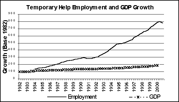
These results are not unexpected. A study by Mangum, Mayall and Nelson (1985) noted that the temporary help industry was quite procyclical long ago, and this has been confirmed by Abraham (1990) and Houseman (2001).
What does this imply about the impact of an economic downturn on at-risk workers in temporary work? Several factors work together to suggest that they will be the first to be laid off. First, the low education levels of this group make them much more vulnerable than other workers. Second, the very nature of temporary work means that there are likely to be very low rates of job-specific skill acquisition, and hence that there are minimal firing costs to employers. Third, since all temporary workers are outside the standard employment relationship (Benner, 1997), there are few penalties associated with layoff. Finally, employers explicitly use non standard work arrangements to buffer against changes in the economy, so it should be expected that this sector will be disproportionately affected by an economic downturn.
All of this taken together suggests that there are likely to be substantial adverse consequences to at-risk temporary help workers in an economic downturn, although the data do not permit this to be quantified.
Where Do We Go From Here?
Just as the main constraints that have been faced in this study have been due to data problems, the main suggestions for future work center around exploiting new and different data sources to analyze the research question. The ideal data source would consist of CPS-quality measures of alternative work arrangements in a relatively large survey dataset that could be linked with long and detailed work histories. This would enable the complex definitions of alternative work arrangements to be examined together with adequate work history controls and varied outcome measures. Such a dataset is currently being developed at the Census Bureau, and if further research were warranted, the next steps could include the following:
- Construction of better quality work histories to structure better comparison groups.
- Inclusion of macroeconomic variables to capture the effect of economic changes on temporary help employment.
- An analysis of the sensitivity of the results to the definition of alternative worker and of at-risk individual.
- An investigation into the reasons for the marked differences in employment growth in temporary help services in establishment and household surveys.
- An investigation into the types of firms that hire at-risk workers and the impact of the firm on worker outcomes.
60. This is confirmed by the distribution of temporary workers in our sample (see Table A.1). Roughly, two-thirds of at-risk temporary work spells were preceded by nonemployment and one third by employment.
Appendices
Data Sources and Definitions
In this appendix, we describe the three data sources used for our study of alternative work arrangements. First, we discuss the Current Population Survey, which is used to address how alternative and non-alternative arrangements differ in their job and worker characteristics. Next, we discuss the Survey of Income and Program Participation, which is used to analyze the effects of working for a temporary agency on subsequent employment and income. Finally, we discuss the Current Employment Statistics, which is used for the limited purpose of examining aggregate growth in employment in the temporary employment industry over time.
The Current Population Survey (CPS)
The CPS is a monthly survey of about 50,000 households conducted by the Bureau of the Census for the Bureau of Labor Statistics. The CPS is the primary source of data on labor force characteristics of the US civilian noninstitutional population. Monthly supplements provide estimates on a variety of topics of interest, including an annual March demographic supplement and a biannual February supplement on alternative work arrangements.(61) This latter supplement is used extensively by papers discussed in the literature review in Chapter 2.
The CPS data appropriate to analyze the characteristics of alternative work arrangement jobs and workers for low-income households come entirely from the February and March Basic Surveys and the supplements to these surveys. Beginning in 1995 and continuing in 1997 and 1999, the February Contingent Worker and Alternative Employment Supplement provides data on the types of work arrangements held by working respondents and on benefits provided by employers. All questions refer to the week prior to the survey date. The March Demographic supplement, administered each year, provides detailed demographic data and information on income levels and receipt of public assistance in the calendar year preceding the survey.
In our analysis of the CPS, we focus on comparing alternative and non-alternative arrangements regardless of income level, and for persons who are at risk of welfare receipt and/or low income, as defined in the next section.
Definitions
As discussed in Chapter 2, the CPS February supplement asks a series of questions that allow us to categorize workers into a variety of alternative work arrangements. The questions ascertain whether the worker is employed on a temporary basis, and if so, the reason for that temporary status. Follow-up questions ask whether the worker's salary is paid by a temporary agency or a contract company, whether the worker is employed on-call, as a day laborer, or is self-employed. Responses to these questions are used to categorize workers as temporary agency and on-call workers.
Although the CPS data allow us to focus on many alternative work arrangements, we focus our analysis on temporary agency and on-call workers. We choose not to focus on the other work arrangements identified in the CPS because the distinctions between regular employment and these types of alternative work arrangements can be narrow. Also, since the core notion of alternative work arrangements describes the relationship between employer and employee (a relationship that differs from standard work arrangements), the nature of temporary agency and on-call work more closely fit our definition of alternative work arrangements for the purposes of this analysis.
In addition to examining the temporary and on-call population as a whole, we also use the CPS to examine the subset of workers who may be at risk of welfare recipiency. The definition of at risk of welfare recipiency is conceptually difficult to pin down. There are different types of public assistance--Aid to Families with Dependent Children/Temporary Assistance for Needy Families, Medicaid, and Food Stamps--and eligibility measures vary by state and family background. Thus, workers with identical earnings, but in different states and in different environments, might well be at different levels of risk of welfare recipiency. Therefore, we use two measures of at-risk workers: those workers who live in households with incomes below 150 percent of the federal poverty level and those who have received public assistance in the previous year (who may not be current welfare recipients).(62)
Sample Size
In the CPS, respondents are included in the survey for four consecutive months, left off for the following eight months, then included again in the survey for four months. This pattern permits us to match observations across different months of the survey and gather information on work arrangements and income at several points in time. Approximately three-fourths of the cases interviewed in the February supplement are also interviewed in March. The actual sample sizes for temporary workers, on-call workers, and regular workers, as well as the subset of public assistance recipients and workers with income below 150 percent of the poverty line are presented in Table 3.1 (see Chapter 3).
The matched data from the February and March surveys from 1995, 1997, and 1999 provide information on current work arrangements and benefits provided by the job held in February as well as receipt of public assistance and income from the previous (even-numbered) year. Almost three-fourths of the observations in each February supplement can be matched to March of the same year. In addition to matching within year, we also considered matching those cases interviewed in February with March of the following year. This would have allowed us to examine impacts of alternative work arrangements on subsequent outcomes. About three-eighths (37.5 percent) of those cases interviewed in the February supplement are also interviewed in February or March of the following year.(63) Matching observations to data from February and/or March of the following year reduces the number of observations by at least half, but allows examination of several outcome measures. Specifically, the supplements for February of 1996, 1998, and 2000 (a year earlier) provide data on whether persons employed in various work arrangements are still employed, and whether they are still employed at the same job. The basic survey for March 1996, 1998, and 2000 provides information on current employment, hours worked, and wages earned from the primary job. However, matching across years resulted in sample sizes that were not large enough to make strong statements about the effects of alternative work arrangements in the at risk population.
Survey of Income and Program Participation (SIPP)
The SIPP is a large-scale survey sponsored by the Census Bureau. For the years 1990 to 1993, fresh national samples were drawn annually. Each fresh annual sample constitutes a panel. Each panel is interviewed 8-10 times; each household is interviewed every fourth month, with successive quarters of the sample interviewed in each month. A 1996 panel with interview data through March 2000 has recently been released, although the longitudinal file is not yet available. Given the resource limitations on this project, we analyzed the 1990, 1991, 1992, and 1993 SIPP panels.
In each wave, the basic questionnaire provides data on the primary jobs held during the previous four months. Questions focus on the two jobs held for the largest number of hours. For these jobs, we know earnings or wage rate, months the job was held, usual hours worked per week, industry, and receipt of health insurance coverage. These variables, together with measures of income and public assistance receipt, are the primary outcome measures for our analysis of the subsequent effects of temporary work. The SIPP supplements the basic survey in each wave with detailed topical modules that provide information including employment and welfare recipiency history. These modules are used to select comparison groups with relatively similar work histories.
Definitions
Our ability to determine alternative work arrangements in the SIPP is limited to identifying workers likely to be employed by temporary help agencies. The industry categorization of the two principal jobs, which is based on a 3-digit SIC code, can be used to learn whether the worker is employed in the temporary help services industry. We categorize a person as being employed in the temporary help services industry if he/she reports that either of the two reported jobs for a given wave is in SIC 736. SIC 736 includes those working for temporary help agencies and employment agencies. The four-digit category for temporary work (which includes some leasing companies) accounts for 89 percent of employment in SIC 736; the category for employment agencies accounts for the remaining 11 percent. Because individuals self-report the SIC code, we expect relatively few persons who work at companies managed by leasing companies will report in SIC 736; they would seem more likely to report the industry in which they work.
One question that arises when using SIC 736 to define temporary help workers is how well SIC 736 identifies agency temporary workers. We examine this using the February Contingent Workers Supplement to the CPS. Using CPS data for 1995 through 1999, we find that 57-70 percent of those in SIC 736 are classified as agency temporaries based on the supplement. In addition, roughly half of those who are identified as agency temporaries in the supplement reported SIC 736 as their industry. A large share of the latter mismatch appears to result from respondents reporting the industry of the place where the temporary agency assigned them to work rather than the industry of the temporary agency. Although these findings suggest caution in using the industry code to define temporary agency workers, we believe the share of agency workers within SIC 736 is high enough that strong differentials associated with agency work will be picked up by our analysis.
Similar to the CPS, in addition to examining temporary workers as a whole, we also use the SIPP to examine the subset of workers who may be at risk of welfare recipiency. We considered definitions of at risk of welfare receipt based on public assistance receipt as well as income relative to the federal poverty level.(64) In the end, we use a definition that balances the need to have enough cases for our analysis with a low enough income cutoff such that the sample members are at significant risk of welfare receipt.
Sample Size
Table A.1 reports the number of spells of temporary work in the 1990-1993 panels of the SIPP. The start of each spell is sampled and used as the base period in the analysis of the effects of temporary work. These numbers include only those temporary workers with data available one year later, a necessary requirement to measure outcomes. In addition to showing sample sizes for the full sample, Table A.1 shows various possible definitions of at risk or low income, including public assistance receipt, income below 150 percent of the poverty line, and income below 200 percent of the poverty line. Given the small sample sizes, we use the broadest of the three definitions--under 200 percent of poverty--for at risk or low income. This serves to balance the need for adequately-sized samples for analysis with the need to focus on a group with sufficiently low income to be at risk of receipt of public assistance.
| Previously Employed | Previously Unemployed | |
|---|---|---|
| Received Public Assistance in Prior Month | 65 | 152 |
| Individuals below 150% of Federal Poverty Level | 143 | 345 |
| Individuals below 200% of Federal Poverty Level | 234 | 425 |
| All Individuals | 648 | 738 |
| Source: SIPP 1990-1993 panels, calculations by the Urban Institute. Note: Sample sizes include all cases that are observed a year after their first month in SIC 736. Poverty figures are based on income in the month prior to employment in SIC 736. |
||
Current Employment Statistics (CES)
The establishment payroll survey, known as the Current Employment Statistics (CES) survey, is administered to a monthly sample of nearly 400,000 business establishments nationwide. Employment is the total number of persons on establishment payrolls employed full or part time who received pay for any part of the pay period which includes the 12th day of the month. Temporary and intermittent employees are included, as are any workers who are on paid sick leave, on paid holiday, or who work during only part of the specified pay period. Data exclude proprietors, self-employed, unpaid family or volunteer workers, farm workers, and domestic workers.(65)
Data from the CES survey are used for only limited analysis in this research because, although they have the advantage of a long time series of data, they lack occupational and demographic detail. More specifically, the CES data are derived from establishment-level surveys and are based on aggregate earnings and hours for workers at each establishment. The only breakout by occupation is for production/non-production workers and the only demographic breakout is for males and females. Consequently, there is no information about workers at risk of welfare recipiency. Also, these series classify workers by establishment--so the definition of a temporary worker, which is based on an industry definition, is conceptually different from that in the CPS. Here, employees themselves may be temporarily assigned to outside customers, but any individual employee may be long term and hold many temporary assignments.
Methodology for SIPP Analysis
The goal of the SIPP analysis is an improved understanding of how temporary work affects subsequent labor market outcomes. Broadly put, we want to estimate how outcomes for persons who begin temporary agency jobs would differ if they had not taken such jobs. The basic approach is to compare the subsequent outcomes for those employed in temporary work with persons who have similar demographic and human capital characteristics, but who did not work for temporary agencies.
To undertake this analysis, we need to define employment in temporary work and identify plausible comparison groups to serve as counterfactuals. Our sample of temporary agency workers includes all instances in which persons begin work for an agency (as either their primary or secondary job) as measured by the SIC code. The decision to focus on the start of spells of temporary work simplifies the modeling of comparison groups and fits naturally with our interest in the effect of decisions to take temporary work rather than other options.
We measure the effect of temporary work relative to both regular employment and nonemployment.(66) To operationalize this, we compare our sample of temporary agency workers to two comparison groups: one matched sample of persons employed in nontemporary work and another of persons not employed. By using two comparison groups, we hope to learn the subsequent effects of obtaining a temporary agency job as compared with being employed at a "regular" job and with not being employed.
The samples are matched based on propensity scores. Roughly put, we estimate a regression model that describes the probability of starting a job with a temporary agency. The predicted probability from such a model is known as a propensity score. We follow recent research (Dehejia & Wahba (1998), Berk and Newton (1985), and Rosenbaum & Rubin (1984)) in choosing comparison group members who match members of our sample of temporary agency workers in their likelihood of becoming a temporary worker, as measured by their propensity score. An alternative would be to match on many characteristics of the individuals (e.g., those included in the regression model). Rosenbaum and Rubin (1984), however, argue that matching on the propensity score, which is a single variable, is nearly as effective as matching on all of the many variables used in the regression model to predict propensity score.
Using the matched comparison groups, we estimate the effect of entering temporary work on several outcomes measured a year later. The outcome measures include employment status, wages, hours worked, health insurance coverage, and receipt of public assistance. These subsequent outcomes are then compared to those for each of the comparison groups, with the differences in outcomes interpreted as the effects of entering temporary work relative to the counterfactual; that is, working at a nontemporary job or not working.
Advantages of Using a Matched Comparison Approach
When considering this type of approach, a natural question arises: Why bother matching the temporary workers and nontemporary workers? Why not simply estimate a regression model that controls for the variables used in matching?
There are several answers to this question. First, use of the matched comparison group brings us (incrementally) closer to a random assignment design, by trying to limit the comparison group to those who match actual temporary workers in their likelihood of taking a temporary job. Second, including persons in a regression analysis with characteristics that indicate that they are very unlikely to be temporary workers adds no additional information to our estimate of the effect of temporary work. Finally, a regression model typically assumes that the relationship between the independent variables and the dependent variable is structurally similar for all members of the sample. Thus, inclusion of many regular workers and non-workers who are dissimilar to temporary workers in the regression could produce spurious results if the relationship between their background characteristics and subsequent outcomes differs from that of those who are similar to temporary workers. Including people dissimilar from the temporary workers in the regression thus may decrease the ability of the regression to accurately estimate how the choice of temporary work affects future employment, for those people for whom this is a reasonable choice.
A good summary of this argument is provided by Dehejia and Wahba (1998) who make the following comments about the methods under consideration:
"[Propensity score methods] reduce the task of controlling for differences in pre-intervention variables between the treatment and the non-experimental comparison groups to controlling for differences in the estimated propensity score (the probability of assignment to treatment, conditional on covariates). It is difficult to control for differences in pre-intervention variables when they are numerous and when the treatment and comparison groups are dissimilar, whereas controlling for the estimated propensity score, a single variable on the unit interval, is a straightforward task. We apply several methods, such as stratification on the propensity score and matching on the propensity score, and show that they result in accurate estimates of the treatment impact." (p.1)
Disadvantages of Using a Matched Comparison Approach
It is worth noting one caveat to this approach. Any conclusions will be based on comparing temporary workers with those most similar to them in their human capital and demographic characteristics. This will be interpreted as an estimate of the impact of temporary work for those who worked for a temporary agency. It can also be reasonably taken as an estimate of the effect of temporary work for those with human capital and demographic characteristics quite similar to those who worked for an agency. However, our estimates cannot provide a measure of the likely effect of temporary work for persons with characteristics quite different from those of the temporary workers or for a broader group, such as all persons on welfare.(67) The conclusions drawn from this analysis, although narrower in scope, are expected to be more reliable and in keeping with the primary research question.
Choice of Temporary Worker and Comparison Groups
In this section, we first discuss the definitions of the temporary worker groups (referred to as treatment groups) and the nontemporary worker comparison groups (referred to as comparison groups). We then discuss the details of the propensity score regression analysis used to construct the comparison groups. The factors used in the propensity score regression analysis are those thought to affect both labor market outcomes and decisions to work for temporary agencies (e.g., demographic characteristics, work history, family structure). Using the constructed comparison groups, we estimate the effects of temporary employment on outcome measures one year after the start of a spell of temporary employment.
Definitions
To obtain a sample of persons beginning temporary work, we select all workers in temporary work (SIC 736) from each month who were not in temporary work in the previous month. The sample is limited to workers between ages 18 and 45. Only those temporary workers whose employment begins at least 12 months before the last month of a panel are included in the analysis, as this allows us to observe outcomes one year later.(68) We include all spells of temporary employment, including multiple spells from the same individual, in our analysis and adjust our model standard errors for correlations among the observations.
This group of temporary workers is further divided into two groups. Prior to entering a temporary job, a person is either employed in nontemporary work or not employed. Since we believe that these two groups may be entering temporary jobs for different reasons, we divide the temporary worker groups into two groups. Treatment Group 1 includes temporary workers who were working in nontemporary employment in the month prior to taking a temporary job. Treatment Group 2 includes temporary workers who were not working in the month prior to taking a temporary job (either unemployed or out of the labor force).
The comparison group contains data for all persons who are not observed in temporary work in any wave of the SIPP.(69) As with the treatment groups, this broad comparison group is divided into two groups. Comparison Group 1 includes persons who were working in the month prior. Comparison Group 2 includes persons who were not working in the month prior (either unemployed or out of the labor force). Thus, based on work status in the prior month, we have two comparison groups.
We further divide Comparison Groups 1 and 2 into two groups based on employment status in the current month, which allows us to estimate the effect of temporary work as compared with both nontemporary employment and nonemployment. Comparison Group 1 is divided into Comparison Group 1A--those employed in the current month--and Comparison Group 1B--those not employed in the current month. Likewise, Comparison Group 2 is divided into Comparison Group 2A--those employed in the current month--and Comparison Group 2B--those not employed in the current month.
In sum, we have the following six treatment and comparison groups:
| В | Prior Month | Current Month |
|---|---|---|
| Treatment Group1 | Employed in Nontemporary Work | Employed in Temporary Work |
| Treatment Group 2 | Not Employed | |
| Comparison Group 1A | Employed in Nontemporary Work | Employed in Nontemporary Work |
| Comparison Group 1B | Not Employed | |
| Comparison Group 2A | Not Employed | Employed in Nontemporary Work |
| Comparison Group 2B | Not Employed |
Constructing Matched Comparison Groups
After defining our treatment and comparison groups, the next step in our methodology is to construct matched comparison groups. That is, we select persons from the comparison group who most closely resemble members of the treatment group on a number of key factors (e.g., demographic characteristics, work and welfare history, family structure). We also control for the timing of the survey interviews, so that the labor market conditions faced by temporary agency workers and the comparison groups will be roughly similar. Samples are matched separately for those who start temporary work following employment and nonemployment, since the relationships in the model are likely to vary with work status.(70)
The basic approach is to use a non-linear regression model to describe who becomes a temporary worker, and then use the predicted probabilities of temporary work from that model as the basis for matching samples. Separate models of the probability of starting a temporary agency job are estimated for those with and without employment in the previous month, allowing the factors affecting the probability to differ for these groups. A multinomial logit model is used for the estimation, to allow for joint estimation of temporary work as compared with the two alternatives: employment and nonemployment.
We estimate two multinomial logit models. The first multinomial logit compares temporary workers who were employed in nontemporary work in the prior month (Treatment Group 1) to nontemporary workers (Comparison Group 1A) and non-workers (Comparison Group1B) who were employed in nontemporary work in the prior month. The second multinomial logit compares temporary workers who were not employed in the prior month (Treatment Group 2) to nontemporary workers (Comparison Group 2A) and non-workers (Comparison Group 2B) not employed in the prior month.
Independent variables for the logit models include:
- Human capital variables, including measures of age, education, consistency of labor market attachment, recentness of time out of the labor market, and recent job training;
- Indicators of a need and ability to work an irregular work schedule, such as number of children, age of youngest child, marital status, number of adults in the household, and measures of recent changes in these variables;
- Other demographic variables that tend to be linked to quality of job such as sex, race, and ethnicity;
- For those employed in the prior month, indicators of employment in a low-wage occupation or industry based on data constructed from the CPS, and a recent wage rate; and
- Measures of the wave and panel of the interview on which the data are based.
The specific measures used are somewhat different for those employed and not employed in the month prior to when we measure temporary work. The complete list of variables used is reported in Table B.1.
Human Capital Variables:
Indicators of need/ability to work flexible work schedule:
Other demographic factors:
Indicators of previous employment
Indicators of low-income status:
Measures of wave and panel:
Indicators of missing data
Human Capital Variables:
Indicators of need/ability to work flexible work schedule:
Other demographic factors:
Indicators of low-income status:
Measures of wave and panel:
Indicators of missing data
|
We then use a two-step matching procedure. First, using the first multinomial logit model estimated above, for each person in the sample, we predict a propensity score--the probability of employment by a temporary agency (Treatment Group 1) as compared with being employed in a nontemporary job (Comparison Group 1A) or not being employed (Comparison Group 1B).
To assess whether the propensity score from the model adequately controls for differences between temporary workers and each of the comparison groups, we compare the mean characteristics of temporary workers (Treatment Group 1), employed (Comparison Group 1A), and nonemployed (Comparison Group 1B) persons with comparable probabilities of temporary work. To do this, we sort the temporary agency cases (Treatment Group 1) by their predicted probability of being a temporary agency worker and find the probabilities associated with each quintile of the distribution. For example, let p80 be the probability associated with the 80th percentile and pmax be the maximum probability for temporary agency cases.
Second, we then compare the mean characteristics of temporary workers (Treatment Group 1) with probabilities in each quintile to those employed/not temporary (Comparison Group 1A) and nonemployed (Comparison Group 1B) persons with probabilities in the same ranges. For instance, we compare the means of variables used in the logit model for those Treatment Group 1, Comparison Group 1A, and Comparison Group 1B cases with probabilities between p80 and pmax. If the model is appropriate for building matched comparison groups, the mean characteristics of these three groups' cases should be similar for cases with probabilities within each chosen range. If, as occurs in our analysis, some characteristics are not similar, we re-estimate the regression model, including higher order functions of the variables that are not similar across the groupings.
After attempting to make the characteristics of the temporary agency workers and the two comparison groups similar within each range of predicted probabilities (e.g., between p80 and pmax), we use the predicted probabilities to create a matched sample. The goal is to choose cases from the Comparison Groups 1A and 1B with the same distribution of propensities as those who start temporary work. The propensity score literature suggests several approaches. The easiest approach is to reweight the data for the comparison group so that a weighted one-fifth of the comparison group members have propensity scores between the cutoffs for each quintile of scores for the temporary agency workers. That is, we weight so that one-fifth of the cases have propensity scores between pmin and p20; a fifth between p20 and p40; etc.(71)
One remaining issue is how to treat data from multiple months for a given case. Multiple observations for the same case are likely correlated and thus need to be accounted for in calculating the standard errors. Among the temporary worker cases, approximately 15 percent have multiple spells. However, because we have relatively few observations of temporary work, we plan to include all of them in our analysis and adjust the standard errors for correlations among the observations.(72)
The comparison groups allow more flexibility as to whether to include multiple observations from a case. Each comparison group must represent all months of the data for which our temporary agency workers are included to avoid misattributing the effects of different labor market conditions to temporary work. However, we expect the data for the comparison group persons to be highly correlated over time and as a consequence, little gain from including multiple observations for the same person in the analysis. Furthermore, because we are aiming to obtain comparison groups roughly similar in size to our sample of temporary workers, we do not anticipate needing multiple observations per case.
Our solution is to randomly include one month of data for each person in the comparison groups. Each observation is assigned to comparison groups according to its employment status in the sampled and previous month. By randomly choosing the selected months, we maintain the representativeness of our sample while ensuring that individuals do not show up more than once.
How Good Is The Comparison?
A commonly accepted method of evaluating the quality of the match is to examine whether or not the comparison and treatment groups differ in their observable characteristics.(73) We therefore perform a series of t-tests that compare the characteristics of the two treatment groups to the characteristics of each of their potential comparison groups. Table B.2 reports the t-statistics derived from comparing the mean of each characteristic of the treatment group with that of the comparison groups for both the full and the low-income samples.
| Comparison Group 2b: Not Employed to Not Employed | Comparison Group 1b: Employed to Not Employed | Comparison Group 2a: Not Employed to Employed | Comparison Group 1a: Employed to Employed | |||||
|---|---|---|---|---|---|---|---|---|
| Full Sample | At-Risk | Full Sample | At-Risk | Full Sample | At-Risk | Full Sample | At-Risk | |
| Demographic Characteristics | ||||||||
| Age | 0.18 | -0.41 | 2.67* | 0.72 | 2.59* | 1.23 | -0.48 | -0.34 |
| White | 2.01* | 1.68 | 1.59 | 1.44 | -0.93 | -0.68 | -0.11 | -0.01 |
| Edlv11 | 0.98 | 1.05 | 5.60* | 3.07* | 1.9 | 0.38 | 0.38 | 0.86 |
| High school | -0.15 | 0.06 | -0.48 | -1.09 | 0.21 | 1.64 | -0.29 | -0.85 |
| College | 0.74 | 0.86 | 4.10* | 3.06* | 1.61 | -0.11 | 0.26 | 0.78 |
| Job training | -0.18 | -0.42 | 2.50* | -0.01 | 1.31 | 1.21 | -0.06 | -0.36 |
| Household Composition | ||||||||
| Married | 0.15 | 0.16 | 0.9 | -0.42 | 0.53 | -0.27 | -0.03 | -0.03 |
| Married and female | -0.26 | -0.07 | 0.57 | -0.04 | 1.89 | 0.14 | 0.54 | 0.11 |
| Change in marital status | -0.86 | -1.18 | 1.49 | 0.28 | -0.31 | -1 | 0.49 | 0.49 |
| Number of children | -1.51 | -1.16 | -2.67* | -1.55 | -0.8 | -0.15 | -0.14 | 0.21 |
| Decrease in number of children | -0.64 | 0.07 | -1.37 | -1.2 | -1.23 | -0.78 | -0.85 | -0.81 |
| Child under one | 0.12 | 0.13 | -1.22 | -0.19 | 0.48 | 0.84 | -0.06 | 0.11 |
| Child under three | -0.66 | -0.42 | -1.53 | -0.12 | 0.44 | 1.05 | -0.35 | 0.25 |
| Child under five | -1.13 | -0.77 | -1.83 | -0.35 | 0.32 | 1.02 | -0.6 | 0.1 |
| Number of adults | 0.65 | -0.64 | -1.52 | -0.92 | -1.69 | -1.85 | -0.42 | -0.15 |
| Increase in number of adults | -0.12 | -0.43 | -3.55* | -1.93 | 1.09 | 0.33 | -0.07 | -0.32 |
| Decrease in number of adults | 0.49 | 0.41 | -1.01 | -0.5 | -4.54* | -4.27* | 0.12 | 0.36 |
| Poverty History | ||||||||
| 100 to 200% of poverty | 0.01 | 0.42 | 0.75 | 3.67* | -1.05 | -0.24 | 0.39 | -0.35 |
| 200% of poverty | 0.79 | 2.47* | 1.64 | -0.77 | ||||
| Work History | ||||||||
| Short term work history | 2.66* | 2.50* | 2.87* | 1.42 | -2.22* | -3.01* | 0.15 | 1.2 |
| Percent of last 10years working | -2.12* | 1.79 | 5.46* | 2.85* | -0.7 | -1.06 | -0.21 | -0.6 |
| Percent of time in welfare | -1.13 | -1.03 | 1.34 | 1.75 | ||||
| Duration unemployment | -3.42* | -2.8 | 1.57 | 1.56 | ||||
| Duration of current job | 1.57 | 1.05 | -2.94* | -1.35 | ||||
| Duration between jobs | -2.48* | -1.08 | -0.34 | -0.41 | ||||
| One job | -2.16* | -0.5 | -0.2 | 0.39 | ||||
| Previous wage | 3.22* | 1.12 | -1.4 | -0.5 | ||||
| Low wage occupation | -2.41* | -1.44 | -0.54 | -0.35 | ||||
| Low wage industry | -2.48* | -0.01 | -0.51 | -0.07 | ||||
| Sample Size | 19,613 | 9,867 | 1,620 | 600 | 1,769 | 1005 | 49,449 | 9,820 |
| Number of Temp Workers | 738 | 425 | 648 | 234 | 738 | 425 | 648 | 234 |
| Source: SIPP 1990-1993 panels, calculations by the Urban Institute. Note: At risk defined as below 200% of family poverty level in month prior to reference month. The comparison group mean is the average of the mean within each of the five quintiles. * Significance of the t-statistics at the 0.05 level. | ||||||||
An analysis of this table reveals that the matching procedure generally worked well in grouping like individuals based on demographic characteristics. There is little significant difference between either set of treatment and comparison groups on the basis of age, sex, race, and education. There is also little difference between the two groups in terms of household structure--marital status, number of children--or changes in the household structure. An exception is in matching temporary workers who were previously employed to those who moved to non-work. For that comparison, many demographic characteristics show significant differences between the comparison and treatment groups.
The only set of characteristics in which the matching procedure consistently performed poorly was on the work history variables: particularly the measures of long- and short-term work history and unemployment duration. This suggests that the models that we use fail to capture the full process by which individuals select into each group, and hence that our estimates are likely to be biased by the degree to which this failure occurs. This is not surprising; it would be difficult to argue that individuals take temporary jobs without the existence of work history factors that affect that choice. The construction of more detailed work histories might well be a solution to controlling for the differences we observe, but this is not possible with the current SIPP dataset.(74) These results, however, do reinforce our earlier suspicion that datasets that are unable to control for such work history measures (such as the CPS) would not be appropriate for use in such an analysis.
61. Bureau of Labor Statistics. "CPS Overview." U.S. DOL/BLS. http://www.bls.census.gov/cps/cpsmain.htm.
62. We define at risk as 150 percent of the federal poverty level rather than 200 percent (our definition of at risk for the SIPP analysis, described below). The lower cutoff is used here because the sample size is adequate for analysis and the lower cutoff provides a sample at greater risk of receipt than is the case with the higher cutoff.
63. However, because the CPS is an addressed-based household survey, the actual number of matched cases is lower, due primarily to individuals changing residences from month to month.
64. Income is based on family income from the month prior to either the start of temporary work or a randomly chosen month (for members of the comparison group), multiplied by 12 to get an annual equivalent. This annualized income is then compared to the federal poverty level.
65. Source: http://www.bls.gov/ces/cesprog.htm.
66. This is particularly important for our analysis of persons at risk of welfare, for whom nonemployment may be at least as likely of an alternative to temporary work as nontemporary work.
67. Our inability to describe the impact of temporary work for welfare recipients results from our relatively small number of temporary agency workers. With a large enough sample of temporary workers, we could sub-sample cases to obtain a distribution of propensity scores similar to that of all welfare recipients. Then we would be more comfortable claiming that we had estimated the effect of temporary work on the full sample of nontemporary workers.
68. We include in our logit analysis of temporary work observations that are missing data a year later in an attempt to include as many cases as possible in predicting who is likely to be employed in temporary work. These cases are excluded from the matching procedure and from the analysis of the effects of temporary work because they lack the outcome information from a year later.
69. To make the sample sizes manageable (and to ensure that they reflect the distribution of survey months), we include data for only one month chosen at random per household in the comparison group. The month is chosen from all months that occur at least 12 months before the end of the panel to ensure a sufficient follow-up period.
70. Separate analyses by previous employment status are also expected to make the experiences of those categorized as temporary workers more homogeneous within a grouping.
71. The quintiles procedure was suggested by Rosenbaum and Rubin (1984). A second approach would be to choose for each temporary agency person, the comparison group person with the most similar propensity score. Both approaches will lead to similar distributions of propensity scores for the two comparison groups and the treatment group of temporary workers. For relatively rare transitions, such as those from employment to nonemployment, the reweighting approach is more feasible for our analysis, since it requires fewer observations than a one-to-one match.
72. As of June 2001, standard errors have not yet been adjusted for non-independence of the cases using STATA's cluster option.
73. While it is possible, and even likely, that the groups differ in their unobservable characteristics--and that this may systematically bias the evaluation of the impact--this problem is endemic to evaluation studies (see, e.g., Heckman et al., 2000), and currently unsolved.
74. A variant of this that was suggested by Rosenbaum and Rubin (1984) is to include in the model interaction terms that capture the variation across sample groups in the effects of work history. For example, work history variables may have different effects on the likelihood of temporary work for older women with no children than for young men. To date, experimentation with such interactions--such as separate models for low- and high-income cases or for men and women did not yield an appreciable improvement in the quality of our match.
References
Abraham, Katherine. "Restructuring the Employment Relationship: The Growth of Market-Mediated Work Arrangements." In K.G. Abraham and R.B. McKersie, eds. New Developments in the Labor Market: Toward a New Institutional Paradigm. 85-120. Cambridge, MA: MIT Press, 1990.
Abraham, Katharine, and Susan K. Taylor. "Firms' use of outside contractors: Theory and evidence" Journal of Labor Economics, Jul 1996; Vol. 14(3).
Autor, David H. "Outsourcing at Will: Unjust Dismissal Doctrine and the Growth of Temporary Help Employment," February, 2000.
Benner, Chris. "Shock Absorbers in the Flexible Economy: The Rise Contingent Employment in Silicon Valley." Working Partnerships USA, 1997.
Berk, R. A. and P. J. Newton, "Does Arrest Really Deter Wife Battery? An Effort to Replicate the Findings of the Minneapolis Spouse Abuse Experiment," American Sociological Review, 50, 253-262, April, 1985.
Brown, Charles. "Minimum Wages, Employment and the Distribution of Income" in The Handbook of Labor Economics edited by Orley Ashenfelter and David Card. Amsterdam: North Holland, 1999: 2102-2159.
Bureau of Labor Statistics. "CPS Overview." U.S. DOL/BLS. <http://www.bls.census.gov/cps/cpsmain.htm>.
Bureau of Labor Statistics. "Contingent and Alternative Employment Arrangements, February 1997." U.S. DOL/BLS. ftp://ftp.bls.gov/pub/news.release/History/conemp.020398.news>. December 1997.
Bureau of Labor Statistics. "Contingent and Alternative Employment Arrangements, February 1999." U.S. DOL/BLS. <ftp://ftp.bls.gov/pub/news.release/History/conemp.12211999.news>. December 1999.
Bureau of Labor Statistics. "New Data on Contingent and Alternative Employment Examined by BLS." U.S. DOL/BLS. <ftp://ftp.bls.gov/pub/news.release/History/conemp.082595.news>. August 1995.
Center for Law and Social Policy and Center on Budget and Policy Priorities. "State Policy Demonstration Project." <www.spdp.org/medicaid/table_3.htm>. January 2000.
Cohany, Sharon R. "Workers in Alternative Employment Arrangements." Monthly Labor Review October 1996.
Cohany, Sharon R. "Workers in Alternative Employment Arrangements: A Second Look." Monthly Labor Review November 1998.
Dehejia, R and S. Wahba, "Causal Effects in Non-Experimental Studies: Re-Evaluating the Evaluation of Training Programs." NBER Working Paper No. W6586, June 1998.
Dickert-Conlin, Stachy and Douglas Holtz-Eakin. "Employee-Based versus Employer-Based Subsidies to Low-Wage Workers: A Public Finance Perspective" JCPR working paper 79 March 1999.
Estevao, Marcello M. and Saul Lach. "The Evolution of the Demand for Temporary Help Supply." NBER Working Paper No. 7427, December 1999.
Farber, Henry S. "Job Creation in the United States: Good Jobs or Bad?" Industrial Relations Section, Princeton University working paper 385, July 1997.
Heckman, James, Justin L. Tobias, and Edward Vytlacil. "Simple Estimators for Treatment Parameters in a Latent Variable Framework with an Application to Estimating the Returns to Schooling." NBER Working Paper 7950, October 2000.
Houseman, Susan N., "Why Employers Use Flexible Staffing Arrangements: Evidence from an Employer Survey." In Industrial and Labor Relations Review, 2001.
Houseman, Susan N. "Flexible Staffing Arrangements: A Report on Temporary Help, On-Call, Direct-Hire Temporary, Leased, Contract Company, and Independent Contractor Employment in the United States." DRAFT, June 1999.
Houseman, Susan N. Temporary, Part-Time, and Contract Employment in the United States: A Report on the W.E. Upjohn Institute's Employer Survey on Flexible Staffing Policies. U.S. Department of Labor. June 1997.
Houseman, Susan N. and Anne E. Polivka. "The Implications of Flexible Staffing Arrangements for Job Stability." Upjohn Institute Staff Working Paper No. 99-056 May 1999.
Hudson, Ken. "No Shortage of "Non-Standard" Jobs" Economic Policy Institute working paper December 1999.
KRA Corporation. Employee Leasing: Implications for State Unemployment Insurance Programs. Unemployment Insurance Service, Department of Labor, 1996.
Lane, Julia. "The Role of Job Turnover in the Low-Wage Labor Market." In The Low-Wage Labor Market: Challenges and Opportunities for Economic Self-Sufficiency, edited by Kelleen Kaye and Demetra Smith Nightingale, pp. 185-198. Urban Institute Press, 2000.
Lee, Dwight R. "Why Is Flexible Employment Increasing?" Journal of Labor Research XVII, no. 4 (Fall 1996): 543-53.
Mangum, G., D. Mayall, and K. Nelson. "The Temporary Help Industry: A Response to the Dula Internal Labor Market." Industrial Labor Relations Review, 38: 599-611, 1985.
Manpower Inc. "Manpower Inc. Facts." Manpower Inc. <http://www.manpower.com/en/story.asp>. 2000.
Moore, Mack A. "The Temporary Help Service Industry: Historical Development, Operation, and Scope." Industrial Labor Relations Review. 1965.
Nardone, Thomas. "CES and CPS Employment Totals: Explaining the Gap." Unpublished manuscript from BLS, 1999.
National Labor Relations Board. M.B. Sturgis, Inc., 331 NLRB No. 173. NLRB: Washington, DC, August 25, 2000.
Pavetti, LaDonna, Michelle Derr, Jacquelyn Anderson, Carole Trippe, and Sidnee Paschal. The Role of Intermediaries in Linking TANF Recipients with Jobs. Mathematica Policy Research, Inc. U.S. DHHS/ASPE, February 2000.
Pawasarat, John. "The Employment Perspective: Jobs Held by the Milwaukee County AFDC Single Parent Population (January 1996-March 1997)." Milwaukee, WI: Employment and Training Institute, December 1997.
Polivka, Anne E. "Contingent and Alternative Work Arrangements, Defined." Monthly Labor Review October 1996a.
Polivka, Anne E. "Into Contingent and Alternative Employment: By Choice?" Monthly Labor Review, October 1996b.
Polivka, Anne E. and Thomas Nardone. "On the Definition of 'Contingent Work'." Monthly Labor Review December 1989.
Rosenbaum, P. R. and D. B. Rubin, "Reducing Bias in Observational Studies Using Subclassification on the Propensity Score," Journal of the American Statistical Association, 79, 516-524, September 1984.
Segal, Lewis M. "Flexible Employment: Composition and Trends." Journal of Labor Research XVII, no. 4, Fall 1996: 523-42.
Segal, Lewis M. and Daniel G. Sullivan. "Wage Differentials for Temporary Services Work: Evidence from Administrative Data," Federal Reserve Bank of Chicago Working Papers Series December 1998.
Segal, Lewis M. and Daniel G. Sullivan. "Temporary Services Employment Durations: Evidence from State UI Data," Federal Reserve Bank of Chicago Working Papers Series December 1997a.
Segal, Lewis M. and Daniel G. Sullivan. "The Growth of Temporary Services Work." Journal of Economic Perspectives Spring 1997b.
Swoboda, Frank. "Temporary Workers Win Benefits Ruling." The Washington Post, August 31 2000, A1.
Theeuwes, Jules, Julia Lane, and David Stevens. "High and Low Earnings Jobs: The Fortunes of Employers and Workers" The Review of Income and Wealth, June 2000: 213-248.
U.S. Department of Labor. "SIC Description for 7363." Occupational Safety and Health Administration. <http://www.osha.gov/cgi-bin/sic/sicser2?7363>. 2000.
U.S. General Accounting Office. "Contingent Workers: Incomes and Benefits Lag Behind Those of Rest of Workforce." GAO/HEHS-00-76, June 2000.